PAC newThis indicator will alert you when a candle goes above or below the price action channel (PAC) but only on the first or second candle after a colour change in candle.
When price is above the price action channel that is a bullish sign, when price is below the PAC that is a bearish sign.
The idea is that a sudden change in price is a cause to investigate further price action moving in that direction so the indicator aims to identify reversal
Scalping strategy that works on 5 min chart and aims to gain 10 pips. Do not act on every signal. Further investigation is required, for example by looking at RSI oversolf and overbought levels. For example, at an oversold area, a buy signal is more valid
ค้นหาในสคริปต์สำหรับ " TABLE "

Table: Forex Central Bank Interest RatesThis tool shows CB Interest Rates for USD, JPY, CAD, CHF, EUR, GBP, NZD, AUD - basically all the majors.
Use override and input your own value if it is changed and I haven't updated the script yet.

Month/Month Percentage % Change, Historical; Seasonal TendencyTable of monthly % changes in Average Price over the last 10 years (or the 10 yrs prior to input year).
Useful for gauging seasonal tendencies of an asset; backtesting monthly volatility and bullish/bearish tendency.
~~User Inputs~~
Choose measure of average: sma(close), sma(ohlc4), vwap(close), vwma(close).
Show last 10yrs, with 10yr average % change, or to just show single year.
Chose input year; with the indicator auto calculating the prior 10 years.
Choose color for labels and size for labels; choose +Ve value color and -Ve value color.
Set 'Daily bars in month': 21 for Forex/Commodities/Indices; 30 for Crypto.
Set precision: decimal places
~~notes~~
-designed for use on Daily timeframe (tradingview is buggy on monthly timeframe calculations, and less precise on weekly timeframe calculations).
-where Current month of year has not occurred yet, will print 9yr average.
-calculates the average change of displayed month compared to the previous month: i.e. Jan22 value represents whole of Jan22 compared to whole of Dec21.
-table displays on the chart over the input year; so for ES, with 2010 selected; shows values from 2001-2010, displaying across 2010-2011 on the chart.
-plots on seperate right hand side scale, so can be shrunk and dragged vertically.
-thanks to @gabx11 for the suggestion which inspired me to write this

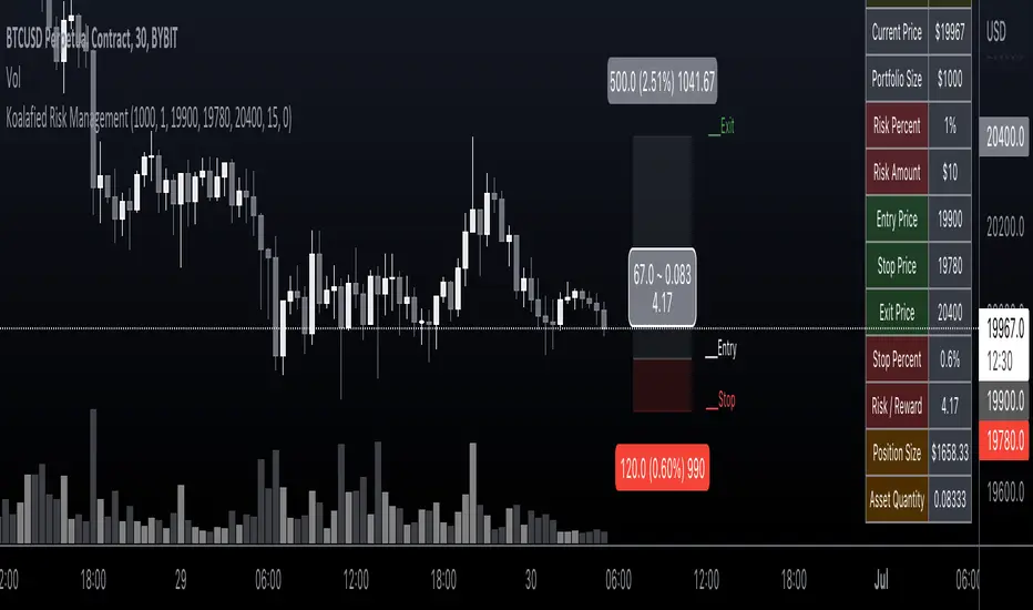
Koalafied Risk ManagementTables and labels/lines showing trade levels and risk/reward. Use to manage trade risk compared to portfolio size.
Initial design optimised for tickers denominated against USD.
Multi-Session High/Low Trackertable that shows rth eth and full weekly range high and low with range difference from high and low

Table ATH and DayQuotes in the middle of a chartJust important things at a glance ..
AlltimeHigh and Daily High/Low

O'Neil Market TimingBill O'Neil Market Timing Indicator - User Guide
Overview
This Pine Script indicator implements William O'Neil's market timing methodology, which assigns one of four distinct states to a market index (such as SPY or QQQ) to help traders identify optimal market conditions for investing. The indicator is designed to work exclusively on Daily timeframe charts.
The Four Market States
The indicator tracks the market through four distinct states, with specific transition rules between them:
1. Confirmed Uptrend (Green)
- Meaning: The market is in a healthy uptrend with institutional support
- Action: Favorable conditions for building positions in leading stocks
- Can transition to: State 2 (Uptrend Under Pressure)
2. Uptrend Under Pressure (Yellow)
- Meaning: The uptrend is showing signs of weakness with increasing distribution
- Action: Be cautious, tighten stops, reduce position sizes
- Can transition to: State 1 (Confirmed Uptrend) or State 3 (Downtrend)
3. Downtrend (Red)
- Meaning: The market is in a confirmed downtrend
- Action: Stay mostly in cash, avoid new purchases
- Can transition to: State 4 (Rally Attempt)
4. Rally Attempt (Pink/Fuchsia)
- Meaning: The market is attempting to bottom and reverse
- Action: Watch for Follow-Through Day to confirm new uptrend
- Can transition to: State 1 (Confirmed Uptrend) or State 3 (Downtrend)
Key Concepts
Distribution Day
A distribution day occurs when:
1. The index closes down by more than the critical percentage (default 0.2%)
2. Volume is higher than the previous day's volume
Distribution days indicate institutional selling and are marked with red triangles on the indicator.
Follow-Through Day
A follow-through day occurs during a Rally Attempt when:
1. The index closes up by more than the critical percentage (default 1.6%)
2. Volume is higher than the previous day's volume
A Follow-Through Day confirms a new uptrend and triggers the transition from Rally Attempt to Confirmed Uptrend.
State Transition Logic
Valid Transitions
The system only allows specific transitions:
- 1 → 2: When distribution days reach the "pressure number" (default 5) within the lookback period (default 25 bars)
- 2 → 1: When distribution days drop below the pressure number
- 2 → 3: When distribution days reach "downtrend number" (default 7) AND price drops by "downtrend criterion" (default 6%) from the lookback high
- 3 → 4: When the market doesn't make a new low for 3 consecutive days
- 4 → 3: When a new low is made, undercutting the downtrend low
- 4 → 1: When a Follow-Through Day occurs during the Rally Attempt
Input Parameters
Distribution Day Parameters
- Distribution Day % Threshold (default 0.2%, range 0.1-2.0%)
- Minimum percentage decline required to qualify as a distribution day. While 0.2% seems to be the canonical number I see in literature about this, I use a much higher threshold (at least 0.5%)
Follow-Through Day Parameters
- Follow-Through Day % Threshold (default 1.6%, range 1.0-2.0%)
- Minimum percentage gain required to qualify as a follow-through day
### State Transition Parameters
- Pressure Number (default 5, range 3-6)
- Number of distribution days needed to transition from Confirmed Uptrend to Uptrend Under Pressure
- Lookback Period (default 25 bars, range 20-30)
- Number of days to count distribution days
- Downtrend Number (default 7, range 4-10)
- Number of distribution days needed (with price drop) to transition to Downtrend
- Downtrend % Drop from High (default 6%, range 5-10%)
- Percentage drop from lookback high required for downtrend confirmation
Visual Settings
- Color customization for each state
- Table position selection (Top Left, Top Right, Bottom Left, Bottom Right)
## How to Use This Indicator
### Installation
1. Open TradingView and navigate to SPY or QQQ (or another major index)
2. **Important**: Switch to the Daily (1D) timeframe
3. Click on "Indicators" at the top of the chart
4. Click "Pine Editor" at the bottom of the screen
5. Copy and paste the Pine Script code
6. Click "Add to Chart"
### Interpretation
**When the indicator shows:**
- **Green (State 1)**: Market is healthy - consider adding quality positions
- **Yellow (State 2)**: Exercise caution - tighten stops, be selective
- **Red (State 3)**: Defensive mode - preserve capital, avoid new buys
- **Pink (State 4)**: Watch closely - prepare for potential Follow-Through Day
### The Information Table
The table displays:
- **Current State**: The current market condition
- **Distribution Days**: Number of distribution days in the lookback period
- **Lookback Period**: Number of bars being analyzed
- **Rally Attempt Day**: (Only in State 4) Days into the current rally attempt
### Visual Elements
1. **State Line**: A stepped line showing the current state (1-4)
2. **Red Triangles**: Mark each distribution day
3. **Horizontal Reference Lines**: Dotted lines marking each state level
4. **Color-Coded Display**: The state line changes color based on the current market condition
## Trading Strategy Guidelines
### In Confirmed Uptrend (State 1)
- Build positions in stocks breaking out of proper bases
- Use normal position sizing
- Focus on stocks showing institutional accumulation
- Hold winners as long as they act properly
### In Uptrend Under Pressure (State 2)
- Take partial profits in extended positions
- Tighten stop losses
- Be more selective with new entries
- Reduce overall exposure
### In Downtrend (State 3)
- Move to cash or maintain very light exposure
- Avoid new purchases
- Focus on preservation of capital
- Use the time for research and watchlist building
### In Rally Attempt (State 4)
- Stay mostly in cash but prepare
- Build a watchlist of strong stocks
- On Day 4+ of the rally attempt, watch for Follow-Through Day
- If FTD occurs, begin cautiously adding positions
## Best Practices
1. **Use with Major Indices**: This indicator works best with SPY, QQQ, or other broad market indices
2. **Daily Timeframe Only**: The indicator is designed for daily bars - do not use on intraday timeframes
3. **Combine with Stock Analysis**: Use the market state as a filter for individual stock decisions
4. **Respect the Signals**: When the market enters Downtrend, reduce exposure regardless of individual stock setups
5. **Monitor Distribution Days**: Pay attention when distribution days accumulate - it's a warning sign
6. **Wait for Follow-Through**: Don't jump back in too early during Rally Attempt - wait for confirmation
## Alert Conditions
The indicator includes built-in alert conditions for:
- State changes (entering any of the four states)
- Distribution Day detection
- Follow-Through Day detection during Rally Attempt
To set up alerts:
1. Click the "Alert" button while the indicator is on your chart
2. Select "O'Neil Market Timing"
3. Choose your desired alert condition
4. Configure notification preferences
## Customization Tips
### For More Sensitive Detection
- Lower the "Pressure Number" to 3-4
- Lower the "Distribution Day % Threshold" to 0.15%
- Reduce the "Downtrend Number" to 5-6
### For More Conservative Detection
- Raise the "Pressure Number" to 6
- Raise the "Distribution Day % Threshold" to 0.3-0.5%
- Increase the "Downtrend Number" to 8-9
### For Different Market Conditions
- **Bull Market**: Consider slightly higher thresholds
- **Bear Market**: Consider slightly lower thresholds
- **Volatile Market**: May need to increase percentage thresholds
## Limitations and Considerations
1. **Not a Crystal Ball**: The indicator identifies conditions but doesn't predict the future
2. **False Signals**: Follow-Through Days can fail - use proper risk management
3. **Whipsaws Possible**: In choppy markets, the indicator may switch states frequently
4. **Confirmation Lag**: By design, there's a lag as the system waits for confirmation
5. **Works Best with Price Action**: Combine with your analysis of individual stocks
## Historical Context
This methodology is based on William J. O'Neil's decades of market research, documented in books like "How to Make Money in Stocks" and through Investor's Business Daily. O'Neil's research showed that:
- Most major market tops are preceded by accumulation of distribution days
- Most successful rallies begin with a Follow-Through Day on Day 4-7 of a rally attempt
- Identifying market state helps prevent buying during unfavorable conditions
## Troubleshooting
**Problem**: Indicator shows "Initializing"
- **Solution**: Let the chart load at least 5 bars to establish the initial state
**Problem**: No distribution day markers appear
- **Solution**: Verify you're on daily timeframe and check if volume data is available
**Problem**: Table not visible
- **Solution**: Check the table position setting and ensure it's not off-screen
**Problem**: State seems to change too frequently
- **Solution**: Increase the lookback period or adjust threshold parameters
## Support and Further Learning
For deeper understanding of this methodology:
- Read "How to Make Money in Stocks" by William J. O'Neil
- Study Investor's Business Daily's "Market Pulse"
- Review historical market tops and bottoms to see the pattern
- Practice identifying distribution days and follow-through days manually
## Version History
**Version 1.0** (November 2025)
- Initial implementation
- Four-state system with proper transitions
- Distribution day detection and marking
- Follow-through day detection
- Customizable parameters
- Information table display
- Alert conditions
---
## Quick Reference Card
| State | Number | Color | Action |
|-------|--------|-------|--------|
| Confirmed Uptrend | 1 | Green | Buy quality setups |
| Uptrend Under Pressure | 2 | Yellow | Tighten stops, be selective |
| Downtrend | 3 | Red | Cash position, no new buys |
| Rally Attempt | 4 | Pink | Watch for Follow-Through Day |
**Distribution Day**: Down > 0.2% on higher volume (red triangle)
**Follow-Through Day**: Up > 1.6% on higher volume during Rally Attempt (triggers State 4→1)
---
*Remember: This indicator is a tool to help identify market conditions. It should be used as part of a comprehensive trading strategy that includes proper risk management, position sizing, and individual stock analysis.*
Also, I created this with the help of an AI coding framework, and I didn't exhaustively test it. I don't actually use this for my own trading, so it's quite possible that it's materially wrong, and that following this will lead to poor investment decisions.. This is "copy left" software, so feel free to alter this to your own tastes, and claim authorship.

Scalper Pro - MA's and Bias - ChartThought I would share this for anybody interested. There is a table in the upper right and you can toggle the moving averages and table on and off as well. Happy Trading!

Quarterly Theory ChecklistThis indicator gives you a fully customizable trading checklist directly on your chart, helping you stay consistent and avoid emotional or impulsive trades.
You can pin the checklist to one specific symbol, so it only appears when you’re analyzing the pair or asset you want to track. Each checklist item has:
A checkbox you can manually toggle
A text label you can customize
Automatic coloring (green check ✔ or red cross ✘)
The indicator also calculates a Trade Score based on how many criteria you’ve checked off.
This score updates live and is color-coded:
Green = 75–100% confidence
Yellow = 50–74%
Red = below 50%
You can choose:
The position of the table
Text size
Header text & colors
Border color
Number of visible checklist rows (1–8)
Enable or disable the Trade Score
Everything is organized inside a clean 2-column checklist table with a polished UI.
Perfect for:
→ System traders
→ Checklists (HTF bias, POIs, confirmations, timing, etc.)
→ Evaluations & trade grading
→ Staying disciplined and rule-based

X ATM Option Ladder Premium (1DTE Dynamic Wings)X ATM Option Ladder Premium is a specialized options-market visualization tool designed for intraday tracking of at-the-money (ATM) option premiums in index ETFs such as QQQ and SPY.The script dynamically identifies the ATM contract on every bar and plots real-time call-versus-put premium differences, with columns for positive/negative diffs and markers (blue dots for positive, red squares for negative) to represent upward price ticks in the option premiums.By analyzing premium levels and direction data from multiple strikes within a dynamic ± range (approximating 0.25 delta wings for 1DTE), the indicator produces a real-time histogram that reflects how premium skew evolves relative to the underlying price.Complementary status tables display the active strike, ladder position, IV-derived wing depth, and warnings when the underlying moves outside the monitored range.Core FeaturesDynamic ATM selection – Each bar automatically maps to the option contract closest to the underlying’s price.Bidirectional premium comparison – Visual separation of call and put premiums (optional columns), with premium diff as the primary histogram and “up” markers highlighting contracts trading above their prior close.Multi-strike ladder analysis – Samples strikes within IV-adjusted wings (±2-5 points typical for 1DTE at 15-25% IV) from the defined center to capture skew and momentum near the money; uses VIX1D for real-time IV approximation.Optimized data calls – Uses tuple requests to minimize request.security() load, enabling a wider ladder within TradingView limits.Session awareness – Restricts processing to the 9:30 AM – 4:15 PM ET option-trading window.Status dashboard – Displays date, active strike, warning flags (“⚠︎ / •outside”), wing parameters (e.g., “±3 (VIX1D=20%)”), and ladder details directly on chart.Use CaseThe indicator is intended for intraday traders and options-premium analysts who want to visualize how short-term pricing dynamics and sentiment migrate across the ATM region as the underlying moves. Typical applications include:Monitoring real-time call/put premium imbalances to detect skew shifts, put-call parity deviations, or implied vol divergences.Identifying premium clustering near the money—where theta decay or gamma effects can signal underlying price acceleration or pinning.Detecting when price exits the monitored ladder (⚠︎ / •outside), signaling a potential regime change or requiring manual recentering.Integrating premium flow into broader volatility or ETF models (e.g., VIX alignment or QQQ/SPY skew confirmation for straddle/strangle trades).Technical NotesStatic-center architecture ensures historical consistency: prior bars remain fixed even after re-centering.Ladder depth is dynamically computed for 1DTE 0.25Δ wings via VIX1D IV (fallback to fixed ±3); capped at ±5 to stay under TradingView’s security-call limits.auto_nudge is enabled to smoothly align the selected lane with the active ATM without requiring user intervention.Indicator is optimized for 1-minute to 5-minute charts; use overlay = false to preserve scale clarity. Manual 1DTE expiry input required (e.g., YYMMDD format).

Universal Ratio Trend Matrix [InvestorUnknown]The Universal Ratio Trend Matrix is designed for trend analysis on asset/asset ratios, supporting up to 40 different assets. Its primary purpose is to help identify which assets are outperforming others within a selection, providing a broad overview of market trends through a matrix of ratios. The indicator automatically expands the matrix based on the number of assets chosen, simplifying the process of comparing multiple assets in terms of performance.
Key features include the ability to choose from a narrow selection of indicators to perform the ratio trend analysis, allowing users to apply well-defined metrics to their comparison.
Drawback: Due to the computational intensity involved in calculating ratios across many assets, the indicator has a limitation related to loading speed. TradingView has time limits for calculations, and for users on the basic (free) plan, this could result in frequent errors due to exceeded time limits. To use the indicator effectively, users with any paid plans should run it on timeframes higher than 8h (the lowest timeframe on which it managed to load with 40 assets), as lower timeframes may not reliably load.
Indicators:
RSI_raw: Simple function to calculate the Relative Strength Index (RSI) of a source (asset price).
RSI_sma: Calculates RSI followed by a Simple Moving Average (SMA).
RSI_ema: Calculates RSI followed by an Exponential Moving Average (EMA).
CCI: Calculates the Commodity Channel Index (CCI).
Fisher: Implements the Fisher Transform to normalize prices.
Utility Functions:
f_remove_exchange_name: Strips the exchange name from asset tickers (e.g., "INDEX:BTCUSD" to "BTCUSD").
f_remove_exchange_name(simple string name) =>
string parts = str.split(name, ":")
string result = array.size(parts) > 1 ? array.get(parts, 1) : name
result
f_get_price: Retrieves the closing price of a given asset ticker using request.security().
f_constant_src: Checks if the source data is constant by comparing multiple consecutive values.
Inputs:
General settings allow users to select the number of tickers for analysis (used_assets) and choose the trend indicator (RSI, CCI, Fisher, etc.).
Table settings customize how trend scores are displayed in terms of text size, header visibility, highlighting options, and top-performing asset identification.
The script includes inputs for up to 40 assets, allowing the user to select various cryptocurrencies (e.g., BTCUSD, ETHUSD, SOLUSD) or other assets for trend analysis.
Price Arrays:
Price values for each asset are stored in variables (price_a1 to price_a40) initialized as na. These prices are updated only for the number of assets specified by the user (used_assets).
Trend scores for each asset are stored in separate arrays
// declare price variables as "na"
var float price_a1 = na, var float price_a2 = na, var float price_a3 = na, var float price_a4 = na, var float price_a5 = na
var float price_a6 = na, var float price_a7 = na, var float price_a8 = na, var float price_a9 = na, var float price_a10 = na
var float price_a11 = na, var float price_a12 = na, var float price_a13 = na, var float price_a14 = na, var float price_a15 = na
var float price_a16 = na, var float price_a17 = na, var float price_a18 = na, var float price_a19 = na, var float price_a20 = na
var float price_a21 = na, var float price_a22 = na, var float price_a23 = na, var float price_a24 = na, var float price_a25 = na
var float price_a26 = na, var float price_a27 = na, var float price_a28 = na, var float price_a29 = na, var float price_a30 = na
var float price_a31 = na, var float price_a32 = na, var float price_a33 = na, var float price_a34 = na, var float price_a35 = na
var float price_a36 = na, var float price_a37 = na, var float price_a38 = na, var float price_a39 = na, var float price_a40 = na
// create "empty" arrays to store trend scores
var a1_array = array.new_int(40, 0), var a2_array = array.new_int(40, 0), var a3_array = array.new_int(40, 0), var a4_array = array.new_int(40, 0)
var a5_array = array.new_int(40, 0), var a6_array = array.new_int(40, 0), var a7_array = array.new_int(40, 0), var a8_array = array.new_int(40, 0)
var a9_array = array.new_int(40, 0), var a10_array = array.new_int(40, 0), var a11_array = array.new_int(40, 0), var a12_array = array.new_int(40, 0)
var a13_array = array.new_int(40, 0), var a14_array = array.new_int(40, 0), var a15_array = array.new_int(40, 0), var a16_array = array.new_int(40, 0)
var a17_array = array.new_int(40, 0), var a18_array = array.new_int(40, 0), var a19_array = array.new_int(40, 0), var a20_array = array.new_int(40, 0)
var a21_array = array.new_int(40, 0), var a22_array = array.new_int(40, 0), var a23_array = array.new_int(40, 0), var a24_array = array.new_int(40, 0)
var a25_array = array.new_int(40, 0), var a26_array = array.new_int(40, 0), var a27_array = array.new_int(40, 0), var a28_array = array.new_int(40, 0)
var a29_array = array.new_int(40, 0), var a30_array = array.new_int(40, 0), var a31_array = array.new_int(40, 0), var a32_array = array.new_int(40, 0)
var a33_array = array.new_int(40, 0), var a34_array = array.new_int(40, 0), var a35_array = array.new_int(40, 0), var a36_array = array.new_int(40, 0)
var a37_array = array.new_int(40, 0), var a38_array = array.new_int(40, 0), var a39_array = array.new_int(40, 0), var a40_array = array.new_int(40, 0)
f_get_price(simple string ticker) =>
request.security(ticker, "", close)
// Prices for each USED asset
f_get_asset_price(asset_number, ticker) =>
if (used_assets >= asset_number)
f_get_price(ticker)
else
na
// overwrite empty variables with the prices if "used_assets" is greater or equal to the asset number
if barstate.isconfirmed // use barstate.isconfirmed to avoid "na prices" and calculation errors that result in empty cells in the table
price_a1 := f_get_asset_price(1, asset1), price_a2 := f_get_asset_price(2, asset2), price_a3 := f_get_asset_price(3, asset3), price_a4 := f_get_asset_price(4, asset4)
price_a5 := f_get_asset_price(5, asset5), price_a6 := f_get_asset_price(6, asset6), price_a7 := f_get_asset_price(7, asset7), price_a8 := f_get_asset_price(8, asset8)
price_a9 := f_get_asset_price(9, asset9), price_a10 := f_get_asset_price(10, asset10), price_a11 := f_get_asset_price(11, asset11), price_a12 := f_get_asset_price(12, asset12)
price_a13 := f_get_asset_price(13, asset13), price_a14 := f_get_asset_price(14, asset14), price_a15 := f_get_asset_price(15, asset15), price_a16 := f_get_asset_price(16, asset16)
price_a17 := f_get_asset_price(17, asset17), price_a18 := f_get_asset_price(18, asset18), price_a19 := f_get_asset_price(19, asset19), price_a20 := f_get_asset_price(20, asset20)
price_a21 := f_get_asset_price(21, asset21), price_a22 := f_get_asset_price(22, asset22), price_a23 := f_get_asset_price(23, asset23), price_a24 := f_get_asset_price(24, asset24)
price_a25 := f_get_asset_price(25, asset25), price_a26 := f_get_asset_price(26, asset26), price_a27 := f_get_asset_price(27, asset27), price_a28 := f_get_asset_price(28, asset28)
price_a29 := f_get_asset_price(29, asset29), price_a30 := f_get_asset_price(30, asset30), price_a31 := f_get_asset_price(31, asset31), price_a32 := f_get_asset_price(32, asset32)
price_a33 := f_get_asset_price(33, asset33), price_a34 := f_get_asset_price(34, asset34), price_a35 := f_get_asset_price(35, asset35), price_a36 := f_get_asset_price(36, asset36)
price_a37 := f_get_asset_price(37, asset37), price_a38 := f_get_asset_price(38, asset38), price_a39 := f_get_asset_price(39, asset39), price_a40 := f_get_asset_price(40, asset40)
Universal Indicator Calculation (f_calc_score):
This function allows switching between different trend indicators (RSI, CCI, Fisher) for flexibility.
It uses a switch-case structure to calculate the indicator score, where a positive trend is denoted by 1 and a negative trend by 0. Each indicator has its own logic to determine whether the asset is trending up or down.
// use switch to allow "universality" in indicator selection
f_calc_score(source, trend_indicator, int_1, int_2) =>
int score = na
if (not f_constant_src(source)) and source > 0.0 // Skip if you are using the same assets for ratio (for example BTC/BTC)
x = switch trend_indicator
"RSI (Raw)" => RSI_raw(source, int_1)
"RSI (SMA)" => RSI_sma(source, int_1, int_2)
"RSI (EMA)" => RSI_ema(source, int_1, int_2)
"CCI" => CCI(source, int_1)
"Fisher" => Fisher(source, int_1)
y = switch trend_indicator
"RSI (Raw)" => x > 50 ? 1 : 0
"RSI (SMA)" => x > 50 ? 1 : 0
"RSI (EMA)" => x > 50 ? 1 : 0
"CCI" => x > 0 ? 1 : 0
"Fisher" => x > x ? 1 : 0
score := y
else
score := 0
score
Array Setting Function (f_array_set):
This function populates an array with scores calculated for each asset based on a base price (p_base) divided by the prices of the individual assets.
It processes multiple assets (up to 40), calling the f_calc_score function for each.
// function to set values into the arrays
f_array_set(a_array, p_base) =>
array.set(a_array, 0, f_calc_score(p_base / price_a1, trend_indicator, int_1, int_2))
array.set(a_array, 1, f_calc_score(p_base / price_a2, trend_indicator, int_1, int_2))
array.set(a_array, 2, f_calc_score(p_base / price_a3, trend_indicator, int_1, int_2))
array.set(a_array, 3, f_calc_score(p_base / price_a4, trend_indicator, int_1, int_2))
array.set(a_array, 4, f_calc_score(p_base / price_a5, trend_indicator, int_1, int_2))
array.set(a_array, 5, f_calc_score(p_base / price_a6, trend_indicator, int_1, int_2))
array.set(a_array, 6, f_calc_score(p_base / price_a7, trend_indicator, int_1, int_2))
array.set(a_array, 7, f_calc_score(p_base / price_a8, trend_indicator, int_1, int_2))
array.set(a_array, 8, f_calc_score(p_base / price_a9, trend_indicator, int_1, int_2))
array.set(a_array, 9, f_calc_score(p_base / price_a10, trend_indicator, int_1, int_2))
array.set(a_array, 10, f_calc_score(p_base / price_a11, trend_indicator, int_1, int_2))
array.set(a_array, 11, f_calc_score(p_base / price_a12, trend_indicator, int_1, int_2))
array.set(a_array, 12, f_calc_score(p_base / price_a13, trend_indicator, int_1, int_2))
array.set(a_array, 13, f_calc_score(p_base / price_a14, trend_indicator, int_1, int_2))
array.set(a_array, 14, f_calc_score(p_base / price_a15, trend_indicator, int_1, int_2))
array.set(a_array, 15, f_calc_score(p_base / price_a16, trend_indicator, int_1, int_2))
array.set(a_array, 16, f_calc_score(p_base / price_a17, trend_indicator, int_1, int_2))
array.set(a_array, 17, f_calc_score(p_base / price_a18, trend_indicator, int_1, int_2))
array.set(a_array, 18, f_calc_score(p_base / price_a19, trend_indicator, int_1, int_2))
array.set(a_array, 19, f_calc_score(p_base / price_a20, trend_indicator, int_1, int_2))
array.set(a_array, 20, f_calc_score(p_base / price_a21, trend_indicator, int_1, int_2))
array.set(a_array, 21, f_calc_score(p_base / price_a22, trend_indicator, int_1, int_2))
array.set(a_array, 22, f_calc_score(p_base / price_a23, trend_indicator, int_1, int_2))
array.set(a_array, 23, f_calc_score(p_base / price_a24, trend_indicator, int_1, int_2))
array.set(a_array, 24, f_calc_score(p_base / price_a25, trend_indicator, int_1, int_2))
array.set(a_array, 25, f_calc_score(p_base / price_a26, trend_indicator, int_1, int_2))
array.set(a_array, 26, f_calc_score(p_base / price_a27, trend_indicator, int_1, int_2))
array.set(a_array, 27, f_calc_score(p_base / price_a28, trend_indicator, int_1, int_2))
array.set(a_array, 28, f_calc_score(p_base / price_a29, trend_indicator, int_1, int_2))
array.set(a_array, 29, f_calc_score(p_base / price_a30, trend_indicator, int_1, int_2))
array.set(a_array, 30, f_calc_score(p_base / price_a31, trend_indicator, int_1, int_2))
array.set(a_array, 31, f_calc_score(p_base / price_a32, trend_indicator, int_1, int_2))
array.set(a_array, 32, f_calc_score(p_base / price_a33, trend_indicator, int_1, int_2))
array.set(a_array, 33, f_calc_score(p_base / price_a34, trend_indicator, int_1, int_2))
array.set(a_array, 34, f_calc_score(p_base / price_a35, trend_indicator, int_1, int_2))
array.set(a_array, 35, f_calc_score(p_base / price_a36, trend_indicator, int_1, int_2))
array.set(a_array, 36, f_calc_score(p_base / price_a37, trend_indicator, int_1, int_2))
array.set(a_array, 37, f_calc_score(p_base / price_a38, trend_indicator, int_1, int_2))
array.set(a_array, 38, f_calc_score(p_base / price_a39, trend_indicator, int_1, int_2))
array.set(a_array, 39, f_calc_score(p_base / price_a40, trend_indicator, int_1, int_2))
a_array
Conditional Array Setting (f_arrayset):
This function checks if the number of used assets is greater than or equal to a specified number before populating the arrays.
// only set values into arrays for USED assets
f_arrayset(asset_number, a_array, p_base) =>
if (used_assets >= asset_number)
f_array_set(a_array, p_base)
else
na
Main Logic
The main logic initializes arrays to store scores for each asset. Each array corresponds to one asset's performance score.
Setting Trend Values: The code calls f_arrayset for each asset, populating the respective arrays with calculated scores based on the asset prices.
Combining Arrays: A combined_array is created to hold all the scores from individual asset arrays. This array facilitates further analysis, allowing for an overview of the performance scores of all assets at once.
// create a combined array (work-around since pinescript doesn't support having array of arrays)
var combined_array = array.new_int(40 * 40, 0)
if barstate.islast
for i = 0 to 39
array.set(combined_array, i, array.get(a1_array, i))
array.set(combined_array, i + (40 * 1), array.get(a2_array, i))
array.set(combined_array, i + (40 * 2), array.get(a3_array, i))
array.set(combined_array, i + (40 * 3), array.get(a4_array, i))
array.set(combined_array, i + (40 * 4), array.get(a5_array, i))
array.set(combined_array, i + (40 * 5), array.get(a6_array, i))
array.set(combined_array, i + (40 * 6), array.get(a7_array, i))
array.set(combined_array, i + (40 * 7), array.get(a8_array, i))
array.set(combined_array, i + (40 * 8), array.get(a9_array, i))
array.set(combined_array, i + (40 * 9), array.get(a10_array, i))
array.set(combined_array, i + (40 * 10), array.get(a11_array, i))
array.set(combined_array, i + (40 * 11), array.get(a12_array, i))
array.set(combined_array, i + (40 * 12), array.get(a13_array, i))
array.set(combined_array, i + (40 * 13), array.get(a14_array, i))
array.set(combined_array, i + (40 * 14), array.get(a15_array, i))
array.set(combined_array, i + (40 * 15), array.get(a16_array, i))
array.set(combined_array, i + (40 * 16), array.get(a17_array, i))
array.set(combined_array, i + (40 * 17), array.get(a18_array, i))
array.set(combined_array, i + (40 * 18), array.get(a19_array, i))
array.set(combined_array, i + (40 * 19), array.get(a20_array, i))
array.set(combined_array, i + (40 * 20), array.get(a21_array, i))
array.set(combined_array, i + (40 * 21), array.get(a22_array, i))
array.set(combined_array, i + (40 * 22), array.get(a23_array, i))
array.set(combined_array, i + (40 * 23), array.get(a24_array, i))
array.set(combined_array, i + (40 * 24), array.get(a25_array, i))
array.set(combined_array, i + (40 * 25), array.get(a26_array, i))
array.set(combined_array, i + (40 * 26), array.get(a27_array, i))
array.set(combined_array, i + (40 * 27), array.get(a28_array, i))
array.set(combined_array, i + (40 * 28), array.get(a29_array, i))
array.set(combined_array, i + (40 * 29), array.get(a30_array, i))
array.set(combined_array, i + (40 * 30), array.get(a31_array, i))
array.set(combined_array, i + (40 * 31), array.get(a32_array, i))
array.set(combined_array, i + (40 * 32), array.get(a33_array, i))
array.set(combined_array, i + (40 * 33), array.get(a34_array, i))
array.set(combined_array, i + (40 * 34), array.get(a35_array, i))
array.set(combined_array, i + (40 * 35), array.get(a36_array, i))
array.set(combined_array, i + (40 * 36), array.get(a37_array, i))
array.set(combined_array, i + (40 * 37), array.get(a38_array, i))
array.set(combined_array, i + (40 * 38), array.get(a39_array, i))
array.set(combined_array, i + (40 * 39), array.get(a40_array, i))
Calculating Sums: A separate array_sums is created to store the total score for each asset by summing the values of their respective score arrays. This allows for easy comparison of overall performance.
Ranking Assets: The final part of the code ranks the assets based on their total scores stored in array_sums. It assigns a rank to each asset, where the asset with the highest score receives the highest rank.
// create array for asset RANK based on array.sum
var ranks = array.new_int(used_assets, 0)
// for loop that calculates the rank of each asset
if barstate.islast
for i = 0 to (used_assets - 1)
int rank = 1
for x = 0 to (used_assets - 1)
if i != x
if array.get(array_sums, i) < array.get(array_sums, x)
rank := rank + 1
array.set(ranks, i, rank)
Dynamic Table Creation
Initialization: The table is initialized with a base structure that includes headers for asset names, scores, and ranks. The headers are set to remain constant, ensuring clarity for users as they interpret the displayed data.
Data Population: As scores are calculated for each asset, the corresponding values are dynamically inserted into the table. This is achieved through a loop that iterates over the scores and ranks stored in the combined_array and array_sums, respectively.
Automatic Extending Mechanism
Variable Asset Count: The code checks the number of assets defined by the user. Instead of hardcoding the number of rows in the table, it uses a variable to determine the extent of the data that needs to be displayed. This allows the table to expand or contract based on the number of assets being analyzed.
Dynamic Row Generation: Within the loop that populates the table, the code appends new rows for each asset based on the current asset count. The structure of each row includes the asset name, its score, and its rank, ensuring that the table remains consistent regardless of how many assets are involved.
// Automatically extending table based on the number of used assets
var table table = table.new(position.bottom_center, 50, 50, color.new(color.black, 100), color.white, 3, color.white, 1)
if barstate.islast
if not hide_head
table.cell(table, 0, 0, "Universal Ratio Trend Matrix", text_color = color.white, bgcolor = #010c3b, text_size = fontSize)
table.merge_cells(table, 0, 0, used_assets + 3, 0)
if not hide_inps
table.cell(table, 0, 1,
text = "Inputs: You are using " + str.tostring(trend_indicator) + ", which takes: " + str.tostring(f_get_input(trend_indicator)),
text_color = color.white, text_size = fontSize), table.merge_cells(table, 0, 1, used_assets + 3, 1)
table.cell(table, 0, 2, "Assets", text_color = color.white, text_size = fontSize, bgcolor = #010c3b)
for x = 0 to (used_assets - 1)
table.cell(table, x + 1, 2, text = str.tostring(array.get(assets, x)), text_color = color.white, bgcolor = #010c3b, text_size = fontSize)
table.cell(table, 0, x + 3, text = str.tostring(array.get(assets, x)), text_color = color.white, bgcolor = f_asset_col(array.get(ranks, x)), text_size = fontSize)
for r = 0 to (used_assets - 1)
for c = 0 to (used_assets - 1)
table.cell(table, c + 1, r + 3, text = str.tostring(array.get(combined_array, c + (r * 40))),
text_color = hl_type == "Text" ? f_get_col(array.get(combined_array, c + (r * 40))) : color.white, text_size = fontSize,
bgcolor = hl_type == "Background" ? f_get_col(array.get(combined_array, c + (r * 40))) : na)
for x = 0 to (used_assets - 1)
table.cell(table, x + 1, x + 3, "", bgcolor = #010c3b)
table.cell(table, used_assets + 1, 2, "", bgcolor = #010c3b)
for x = 0 to (used_assets - 1)
table.cell(table, used_assets + 1, x + 3, "==>", text_color = color.white)
table.cell(table, used_assets + 2, 2, "SUM", text_color = color.white, text_size = fontSize, bgcolor = #010c3b)
table.cell(table, used_assets + 3, 2, "RANK", text_color = color.white, text_size = fontSize, bgcolor = #010c3b)
for x = 0 to (used_assets - 1)
table.cell(table, used_assets + 2, x + 3,
text = str.tostring(array.get(array_sums, x)),
text_color = color.white, text_size = fontSize,
bgcolor = f_highlight_sum(array.get(array_sums, x), array.get(ranks, x)))
table.cell(table, used_assets + 3, x + 3,
text = str.tostring(array.get(ranks, x)),
text_color = color.white, text_size = fontSize,
bgcolor = f_highlight_rank(array.get(ranks, x)))

Markov Chain [3D] | FractalystWhat exactly is a Markov Chain?
This indicator uses a Markov Chain model to analyze, quantify, and visualize the transitions between market regimes (Bull, Bear, Neutral) on your chart. It dynamically detects these regimes in real-time, calculates transition probabilities, and displays them as animated 3D spheres and arrows, giving traders intuitive insight into current and future market conditions.
How does a Markov Chain work, and how should I read this spheres-and-arrows diagram?
Think of three weather modes: Sunny, Rainy, Cloudy.
Each sphere is one mode. The loop on a sphere means “stay the same next step” (e.g., Sunny again tomorrow).
The arrows leaving a sphere show where things usually go next if they change (e.g., Sunny moving to Cloudy).
Some paths matter more than others. A more prominent loop means the current mode tends to persist. A more prominent outgoing arrow means a change to that destination is the usual next step.
Direction isn’t symmetric: moving Sunny→Cloudy can behave differently than Cloudy→Sunny.
Now relabel the spheres to markets: Bull, Bear, Neutral.
Spheres: market regimes (uptrend, downtrend, range).
Self‑loop: tendency for the current regime to continue on the next bar.
Arrows: the most common next regime if a switch happens.
How to read: Start at the sphere that matches current bar state. If the loop stands out, expect continuation. If one outgoing path stands out, that switch is the typical next step. Opposite directions can differ (Bear→Neutral doesn’t have to match Neutral→Bear).
What states and transitions are shown?
The three market states visualized are:
Bullish (Bull): Upward or strong-market regime.
Bearish (Bear): Downward or weak-market regime.
Neutral: Sideways or range-bound regime.
Bidirectional animated arrows and probability labels show how likely the market is to move from one regime to another (e.g., Bull → Bear or Neutral → Bull).
How does the regime detection system work?
You can use either built-in price returns (based on adaptive Z-score normalization) or supply three custom indicators (such as volume, oscillators, etc.).
Values are statistically normalized (Z-scored) over a configurable lookback period.
The normalized outputs are classified into Bull, Bear, or Neutral zones.
If using three indicators, their regime signals are averaged and smoothed for robustness.
How are transition probabilities calculated?
On every confirmed bar, the algorithm tracks the sequence of detected market states, then builds a rolling window of transitions.
The code maintains a transition count matrix for all regime pairs (e.g., Bull → Bear).
Transition probabilities are extracted for each possible state change using Laplace smoothing for numerical stability, and frequently updated in real-time.
What is unique about the visualization?
3D animated spheres represent each regime and change visually when active.
Animated, bidirectional arrows reveal transition probabilities and allow you to see both dominant and less likely regime flows.
Particles (moving dots) animate along the arrows, enhancing the perception of regime flow direction and speed.
All elements dynamically update with each new price bar, providing a live market map in an intuitive, engaging format.
Can I use custom indicators for regime classification?
Yes! Enable the "Custom Indicators" switch and select any three chart series as inputs. These will be normalized and combined (each with equal weight), broadening the regime classification beyond just price-based movement.
What does the “Lookback Period” control?
Lookback Period (default: 100) sets how much historical data builds the probability matrix. Shorter periods adapt faster to regime changes but may be noisier. Longer periods are more stable but slower to adapt.
How is this different from a Hidden Markov Model (HMM)?
It sets the window for both regime detection and probability calculations. Lower values make the system more reactive, but potentially noisier. Higher values smooth estimates and make the system more robust.
How is this Markov Chain different from a Hidden Markov Model (HMM)?
Markov Chain (as here): All market regimes (Bull, Bear, Neutral) are directly observable on the chart. The transition matrix is built from actual detected regimes, keeping the model simple and interpretable.
Hidden Markov Model: The actual regimes are unobservable ("hidden") and must be inferred from market output or indicator "emissions" using statistical learning algorithms. HMMs are more complex, can capture more subtle structure, but are harder to visualize and require additional machine learning steps for training.
A standard Markov Chain models transitions between observable states using a simple transition matrix, while a Hidden Markov Model assumes the true states are hidden (latent) and must be inferred from observable “emissions” like price or volume data. In practical terms, a Markov Chain is transparent and easier to implement and interpret; an HMM is more expressive but requires statistical inference to estimate hidden states from data.
Markov Chain: states are observable; you directly count or estimate transition probabilities between visible states. This makes it simpler, faster, and easier to validate and tune.
HMM: states are hidden; you only observe emissions generated by those latent states. Learning involves machine learning/statistical algorithms (commonly Baum–Welch/EM for training and Viterbi for decoding) to infer both the transition dynamics and the most likely hidden state sequence from data.
How does the indicator avoid “repainting” or look-ahead bias?
All regime changes and matrix updates happen only on confirmed (closed) bars, so no future data is leaked, ensuring reliable real-time operation.
Are there practical tuning tips?
Tune the Lookback Period for your asset/timeframe: shorter for fast markets, longer for stability.
Use custom indicators if your asset has unique regime drivers.
Watch for rapid changes in transition probabilities as early warning of a possible regime shift.
Who is this indicator for?
Quants and quantitative researchers exploring probabilistic market modeling, especially those interested in regime-switching dynamics and Markov models.
Programmers and system developers who need a probabilistic regime filter for systematic and algorithmic backtesting:
The Markov Chain indicator is ideally suited for programmatic integration via its bias output (1 = Bull, 0 = Neutral, -1 = Bear).
Although the visualization is engaging, the core output is designed for automated, rules-based workflows—not for discretionary/manual trading decisions.
Developers can connect the indicator’s output directly to their Pine Script logic (using input.source()), allowing rapid and robust backtesting of regime-based strategies.
It acts as a plug-and-play regime filter: simply plug the bias output into your entry/exit logic, and you have a scientifically robust, probabilistically-derived signal for filtering, timing, position sizing, or risk regimes.
The MC's output is intentionally "trinary" (1/0/-1), focusing on clear regime states for unambiguous decision-making in code. If you require nuanced, multi-probability or soft-label state vectors, consider expanding the indicator or stacking it with a probability-weighted logic layer in your scripting.
Because it avoids subjectivity, this approach is optimal for systematic quants, algo developers building backtested, repeatable strategies based on probabilistic regime analysis.
What's the mathematical foundation behind this?
The mathematical foundation behind this Markov Chain indicator—and probabilistic regime detection in finance—draws from two principal models: the (standard) Markov Chain and the Hidden Markov Model (HMM).
How to use this indicator programmatically?
The Markov Chain indicator automatically exports a bias value (+1 for Bullish, -1 for Bearish, 0 for Neutral) as a plot visible in the Data Window. This allows you to integrate its regime signal into your own scripts and strategies for backtesting, automation, or live trading.
Step-by-Step Integration with Pine Script (input.source)
Add the Markov Chain indicator to your chart.
This must be done first, since your custom script will "pull" the bias signal from the indicator's plot.
In your strategy, create an input using input.source()
Example:
//@version=5
strategy("MC Bias Strategy Example")
mcBias = input.source(close, "MC Bias Source")
After saving, go to your script’s settings. For the “MC Bias Source” input, select the plot/output of the Markov Chain indicator (typically its bias plot).
Use the bias in your trading logic
Example (long only on Bull, flat otherwise):
if mcBias == 1
strategy.entry("Long", strategy.long)
else
strategy.close("Long")
For more advanced workflows, combine mcBias with additional filters or trailing stops.
How does this work behind-the-scenes?
TradingView’s input.source() lets you use any plot from another indicator as a real-time, “live” data feed in your own script (source).
The selected bias signal is available to your Pine code as a variable, enabling logical decisions based on regime (trend-following, mean-reversion, etc.).
This enables powerful strategy modularity : decouple regime detection from entry/exit logic, allowing fast experimentation without rewriting core signal code.
Integrating 45+ Indicators with Your Markov Chain — How & Why
The Enhanced Custom Indicators Export script exports a massive suite of over 45 technical indicators—ranging from classic momentum (RSI, MACD, Stochastic, etc.) to trend, volume, volatility, and oscillator tools—all pre-calculated, centered/scaled, and available as plots.
// Enhanced Custom Indicators Export - 45 Technical Indicators
// Comprehensive technical analysis suite for advanced market regime detection
//@version=6
indicator('Enhanced Custom Indicators Export | Fractalyst', shorttitle='Enhanced CI Export', overlay=false, scale=scale.right, max_labels_count=500, max_lines_count=500)
// |----- Input Parameters -----| //
momentum_group = "Momentum Indicators"
trend_group = "Trend Indicators"
volume_group = "Volume Indicators"
volatility_group = "Volatility Indicators"
oscillator_group = "Oscillator Indicators"
display_group = "Display Settings"
// Common lengths
length_14 = input.int(14, "Standard Length (14)", minval=1, maxval=100, group=momentum_group)
length_20 = input.int(20, "Medium Length (20)", minval=1, maxval=200, group=trend_group)
length_50 = input.int(50, "Long Length (50)", minval=1, maxval=200, group=trend_group)
// Display options
show_table = input.bool(true, "Show Values Table", group=display_group)
table_size = input.string("Small", "Table Size", options= , group=display_group)
// |----- MOMENTUM INDICATORS (15 indicators) -----| //
// 1. RSI (Relative Strength Index)
rsi_14 = ta.rsi(close, length_14)
rsi_centered = rsi_14 - 50
// 2. Stochastic Oscillator
stoch_k = ta.stoch(close, high, low, length_14)
stoch_d = ta.sma(stoch_k, 3)
stoch_centered = stoch_k - 50
// 3. Williams %R
williams_r = ta.stoch(close, high, low, length_14) - 100
// 4. MACD (Moving Average Convergence Divergence)
= ta.macd(close, 12, 26, 9)
// 5. Momentum (Rate of Change)
momentum = ta.mom(close, length_14)
momentum_pct = (momentum / close ) * 100
// 6. Rate of Change (ROC)
roc = ta.roc(close, length_14)
// 7. Commodity Channel Index (CCI)
cci = ta.cci(close, length_20)
// 8. Money Flow Index (MFI)
mfi = ta.mfi(close, length_14)
mfi_centered = mfi - 50
// 9. Awesome Oscillator (AO)
ao = ta.sma(hl2, 5) - ta.sma(hl2, 34)
// 10. Accelerator Oscillator (AC)
ac = ao - ta.sma(ao, 5)
// 11. Chande Momentum Oscillator (CMO)
cmo = ta.cmo(close, length_14)
// 12. Detrended Price Oscillator (DPO)
dpo = close - ta.sma(close, length_20)
// 13. Price Oscillator (PPO)
ppo = ta.sma(close, 12) - ta.sma(close, 26)
ppo_pct = (ppo / ta.sma(close, 26)) * 100
// 14. TRIX
trix_ema1 = ta.ema(close, length_14)
trix_ema2 = ta.ema(trix_ema1, length_14)
trix_ema3 = ta.ema(trix_ema2, length_14)
trix = ta.roc(trix_ema3, 1) * 10000
// 15. Klinger Oscillator
klinger = ta.ema(volume * (high + low + close) / 3, 34) - ta.ema(volume * (high + low + close) / 3, 55)
// 16. Fisher Transform
fisher_hl2 = 0.5 * (hl2 - ta.lowest(hl2, 10)) / (ta.highest(hl2, 10) - ta.lowest(hl2, 10)) - 0.25
fisher = 0.5 * math.log((1 + fisher_hl2) / (1 - fisher_hl2))
// 17. Stochastic RSI
stoch_rsi = ta.stoch(rsi_14, rsi_14, rsi_14, length_14)
stoch_rsi_centered = stoch_rsi - 50
// 18. Relative Vigor Index (RVI)
rvi_num = ta.swma(close - open)
rvi_den = ta.swma(high - low)
rvi = rvi_den != 0 ? rvi_num / rvi_den : 0
// 19. Balance of Power (BOP)
bop = (close - open) / (high - low)
// |----- TREND INDICATORS (10 indicators) -----| //
// 20. Simple Moving Average Momentum
sma_20 = ta.sma(close, length_20)
sma_momentum = ((close - sma_20) / sma_20) * 100
// 21. Exponential Moving Average Momentum
ema_20 = ta.ema(close, length_20)
ema_momentum = ((close - ema_20) / ema_20) * 100
// 22. Parabolic SAR
sar = ta.sar(0.02, 0.02, 0.2)
sar_trend = close > sar ? 1 : -1
// 23. Linear Regression Slope
lr_slope = ta.linreg(close, length_20, 0) - ta.linreg(close, length_20, 1)
// 24. Moving Average Convergence (MAC)
mac = ta.sma(close, 10) - ta.sma(close, 30)
// 25. Trend Intensity Index (TII)
tii_sum = 0.0
for i = 1 to length_20
tii_sum += close > close ? 1 : 0
tii = (tii_sum / length_20) * 100
// 26. Ichimoku Cloud Components
ichimoku_tenkan = (ta.highest(high, 9) + ta.lowest(low, 9)) / 2
ichimoku_kijun = (ta.highest(high, 26) + ta.lowest(low, 26)) / 2
ichimoku_signal = ichimoku_tenkan > ichimoku_kijun ? 1 : -1
// 27. MESA Adaptive Moving Average (MAMA)
mama_alpha = 2.0 / (length_20 + 1)
mama = ta.ema(close, length_20)
mama_momentum = ((close - mama) / mama) * 100
// 28. Zero Lag Exponential Moving Average (ZLEMA)
zlema_lag = math.round((length_20 - 1) / 2)
zlema_data = close + (close - close )
zlema = ta.ema(zlema_data, length_20)
zlema_momentum = ((close - zlema) / zlema) * 100
// |----- VOLUME INDICATORS (6 indicators) -----| //
// 29. On-Balance Volume (OBV)
obv = ta.obv
// 30. Volume Rate of Change (VROC)
vroc = ta.roc(volume, length_14)
// 31. Price Volume Trend (PVT)
pvt = ta.pvt
// 32. Negative Volume Index (NVI)
nvi = 0.0
nvi := volume < volume ? nvi + ((close - close ) / close ) * nvi : nvi
// 33. Positive Volume Index (PVI)
pvi = 0.0
pvi := volume > volume ? pvi + ((close - close ) / close ) * pvi : pvi
// 34. Volume Oscillator
vol_osc = ta.sma(volume, 5) - ta.sma(volume, 10)
// 35. Ease of Movement (EOM)
eom_distance = high - low
eom_box_height = volume / 1000000
eom = eom_box_height != 0 ? eom_distance / eom_box_height : 0
eom_sma = ta.sma(eom, length_14)
// 36. Force Index
force_index = volume * (close - close )
force_index_sma = ta.sma(force_index, length_14)
// |----- VOLATILITY INDICATORS (10 indicators) -----| //
// 37. Average True Range (ATR)
atr = ta.atr(length_14)
atr_pct = (atr / close) * 100
// 38. Bollinger Bands Position
bb_basis = ta.sma(close, length_20)
bb_dev = 2.0 * ta.stdev(close, length_20)
bb_upper = bb_basis + bb_dev
bb_lower = bb_basis - bb_dev
bb_position = bb_dev != 0 ? (close - bb_basis) / bb_dev : 0
bb_width = bb_dev != 0 ? (bb_upper - bb_lower) / bb_basis * 100 : 0
// 39. Keltner Channels Position
kc_basis = ta.ema(close, length_20)
kc_range = ta.ema(ta.tr, length_20)
kc_upper = kc_basis + (2.0 * kc_range)
kc_lower = kc_basis - (2.0 * kc_range)
kc_position = kc_range != 0 ? (close - kc_basis) / kc_range : 0
// 40. Donchian Channels Position
dc_upper = ta.highest(high, length_20)
dc_lower = ta.lowest(low, length_20)
dc_basis = (dc_upper + dc_lower) / 2
dc_position = (dc_upper - dc_lower) != 0 ? (close - dc_basis) / (dc_upper - dc_lower) : 0
// 41. Standard Deviation
std_dev = ta.stdev(close, length_20)
std_dev_pct = (std_dev / close) * 100
// 42. Relative Volatility Index (RVI)
rvi_up = ta.stdev(close > close ? close : 0, length_14)
rvi_down = ta.stdev(close < close ? close : 0, length_14)
rvi_total = rvi_up + rvi_down
rvi_volatility = rvi_total != 0 ? (rvi_up / rvi_total) * 100 : 50
// 43. Historical Volatility
hv_returns = math.log(close / close )
hv = ta.stdev(hv_returns, length_20) * math.sqrt(252) * 100
// 44. Garman-Klass Volatility
gk_vol = math.log(high/low) * math.log(high/low) - (2*math.log(2)-1) * math.log(close/open) * math.log(close/open)
gk_volatility = math.sqrt(ta.sma(gk_vol, length_20)) * 100
// 45. Parkinson Volatility
park_vol = math.log(high/low) * math.log(high/low)
parkinson = math.sqrt(ta.sma(park_vol, length_20) / (4 * math.log(2))) * 100
// 46. Rogers-Satchell Volatility
rs_vol = math.log(high/close) * math.log(high/open) + math.log(low/close) * math.log(low/open)
rogers_satchell = math.sqrt(ta.sma(rs_vol, length_20)) * 100
// |----- OSCILLATOR INDICATORS (5 indicators) -----| //
// 47. Elder Ray Index
elder_bull = high - ta.ema(close, 13)
elder_bear = low - ta.ema(close, 13)
elder_power = elder_bull + elder_bear
// 48. Schaff Trend Cycle (STC)
stc_macd = ta.ema(close, 23) - ta.ema(close, 50)
stc_k = ta.stoch(stc_macd, stc_macd, stc_macd, 10)
stc_d = ta.ema(stc_k, 3)
stc = ta.stoch(stc_d, stc_d, stc_d, 10)
// 49. Coppock Curve
coppock_roc1 = ta.roc(close, 14)
coppock_roc2 = ta.roc(close, 11)
coppock = ta.wma(coppock_roc1 + coppock_roc2, 10)
// 50. Know Sure Thing (KST)
kst_roc1 = ta.roc(close, 10)
kst_roc2 = ta.roc(close, 15)
kst_roc3 = ta.roc(close, 20)
kst_roc4 = ta.roc(close, 30)
kst = ta.sma(kst_roc1, 10) + 2*ta.sma(kst_roc2, 10) + 3*ta.sma(kst_roc3, 10) + 4*ta.sma(kst_roc4, 15)
// 51. Percentage Price Oscillator (PPO)
ppo_line = ((ta.ema(close, 12) - ta.ema(close, 26)) / ta.ema(close, 26)) * 100
ppo_signal = ta.ema(ppo_line, 9)
ppo_histogram = ppo_line - ppo_signal
// |----- PLOT MAIN INDICATORS -----| //
// Plot key momentum indicators
plot(rsi_centered, title="01_RSI_Centered", color=color.purple, linewidth=1)
plot(stoch_centered, title="02_Stoch_Centered", color=color.blue, linewidth=1)
plot(williams_r, title="03_Williams_R", color=color.red, linewidth=1)
plot(macd_histogram, title="04_MACD_Histogram", color=color.orange, linewidth=1)
plot(cci, title="05_CCI", color=color.green, linewidth=1)
// Plot trend indicators
plot(sma_momentum, title="06_SMA_Momentum", color=color.navy, linewidth=1)
plot(ema_momentum, title="07_EMA_Momentum", color=color.maroon, linewidth=1)
plot(sar_trend, title="08_SAR_Trend", color=color.teal, linewidth=1)
plot(lr_slope, title="09_LR_Slope", color=color.lime, linewidth=1)
plot(mac, title="10_MAC", color=color.fuchsia, linewidth=1)
// Plot volatility indicators
plot(atr_pct, title="11_ATR_Pct", color=color.yellow, linewidth=1)
plot(bb_position, title="12_BB_Position", color=color.aqua, linewidth=1)
plot(kc_position, title="13_KC_Position", color=color.olive, linewidth=1)
plot(std_dev_pct, title="14_StdDev_Pct", color=color.silver, linewidth=1)
plot(bb_width, title="15_BB_Width", color=color.gray, linewidth=1)
// Plot volume indicators
plot(vroc, title="16_VROC", color=color.blue, linewidth=1)
plot(eom_sma, title="17_EOM", color=color.red, linewidth=1)
plot(vol_osc, title="18_Vol_Osc", color=color.green, linewidth=1)
plot(force_index_sma, title="19_Force_Index", color=color.orange, linewidth=1)
plot(obv, title="20_OBV", color=color.purple, linewidth=1)
// Plot additional oscillators
plot(ao, title="21_Awesome_Osc", color=color.navy, linewidth=1)
plot(cmo, title="22_CMO", color=color.maroon, linewidth=1)
plot(dpo, title="23_DPO", color=color.teal, linewidth=1)
plot(trix, title="24_TRIX", color=color.lime, linewidth=1)
plot(fisher, title="25_Fisher", color=color.fuchsia, linewidth=1)
// Plot more momentum indicators
plot(mfi_centered, title="26_MFI_Centered", color=color.yellow, linewidth=1)
plot(ac, title="27_AC", color=color.aqua, linewidth=1)
plot(ppo_pct, title="28_PPO_Pct", color=color.olive, linewidth=1)
plot(stoch_rsi_centered, title="29_StochRSI_Centered", color=color.silver, linewidth=1)
plot(klinger, title="30_Klinger", color=color.gray, linewidth=1)
// Plot trend continuation
plot(tii, title="31_TII", color=color.blue, linewidth=1)
plot(ichimoku_signal, title="32_Ichimoku_Signal", color=color.red, linewidth=1)
plot(mama_momentum, title="33_MAMA_Momentum", color=color.green, linewidth=1)
plot(zlema_momentum, title="34_ZLEMA_Momentum", color=color.orange, linewidth=1)
plot(bop, title="35_BOP", color=color.purple, linewidth=1)
// Plot volume continuation
plot(nvi, title="36_NVI", color=color.navy, linewidth=1)
plot(pvi, title="37_PVI", color=color.maroon, linewidth=1)
plot(momentum_pct, title="38_Momentum_Pct", color=color.teal, linewidth=1)
plot(roc, title="39_ROC", color=color.lime, linewidth=1)
plot(rvi, title="40_RVI", color=color.fuchsia, linewidth=1)
// Plot volatility continuation
plot(dc_position, title="41_DC_Position", color=color.yellow, linewidth=1)
plot(rvi_volatility, title="42_RVI_Volatility", color=color.aqua, linewidth=1)
plot(hv, title="43_Historical_Vol", color=color.olive, linewidth=1)
plot(gk_volatility, title="44_GK_Volatility", color=color.silver, linewidth=1)
plot(parkinson, title="45_Parkinson_Vol", color=color.gray, linewidth=1)
// Plot final oscillators
plot(rogers_satchell, title="46_RS_Volatility", color=color.blue, linewidth=1)
plot(elder_power, title="47_Elder_Power", color=color.red, linewidth=1)
plot(stc, title="48_STC", color=color.green, linewidth=1)
plot(coppock, title="49_Coppock", color=color.orange, linewidth=1)
plot(kst, title="50_KST", color=color.purple, linewidth=1)
// Plot final indicators
plot(ppo_histogram, title="51_PPO_Histogram", color=color.navy, linewidth=1)
plot(pvt, title="52_PVT", color=color.maroon, linewidth=1)
// |----- Reference Lines -----| //
hline(0, "Zero Line", color=color.gray, linestyle=hline.style_dashed, linewidth=1)
hline(50, "Midline", color=color.gray, linestyle=hline.style_dotted, linewidth=1)
hline(-50, "Lower Midline", color=color.gray, linestyle=hline.style_dotted, linewidth=1)
hline(25, "Upper Threshold", color=color.gray, linestyle=hline.style_dotted, linewidth=1)
hline(-25, "Lower Threshold", color=color.gray, linestyle=hline.style_dotted, linewidth=1)
// |----- Enhanced Information Table -----| //
if show_table and barstate.islast
table_position = position.top_right
table_text_size = table_size == "Tiny" ? size.tiny : table_size == "Small" ? size.small : size.normal
var table info_table = table.new(table_position, 3, 18, bgcolor=color.new(color.white, 85), border_width=1, border_color=color.gray)
// Headers
table.cell(info_table, 0, 0, 'Category', text_color=color.black, text_size=table_text_size, bgcolor=color.new(color.blue, 70))
table.cell(info_table, 1, 0, 'Indicator', text_color=color.black, text_size=table_text_size, bgcolor=color.new(color.blue, 70))
table.cell(info_table, 2, 0, 'Value', text_color=color.black, text_size=table_text_size, bgcolor=color.new(color.blue, 70))
// Key Momentum Indicators
table.cell(info_table, 0, 1, 'MOMENTUM', text_color=color.purple, text_size=table_text_size, bgcolor=color.new(color.purple, 90))
table.cell(info_table, 1, 1, 'RSI Centered', text_color=color.purple, text_size=table_text_size)
table.cell(info_table, 2, 1, str.tostring(rsi_centered, '0.00'), text_color=color.purple, text_size=table_text_size)
table.cell(info_table, 0, 2, '', text_color=color.blue, text_size=table_text_size)
table.cell(info_table, 1, 2, 'Stoch Centered', text_color=color.blue, text_size=table_text_size)
table.cell(info_table, 2, 2, str.tostring(stoch_centered, '0.00'), text_color=color.blue, text_size=table_text_size)
table.cell(info_table, 0, 3, '', text_color=color.red, text_size=table_text_size)
table.cell(info_table, 1, 3, 'Williams %R', text_color=color.red, text_size=table_text_size)
table.cell(info_table, 2, 3, str.tostring(williams_r, '0.00'), text_color=color.red, text_size=table_text_size)
table.cell(info_table, 0, 4, '', text_color=color.orange, text_size=table_text_size)
table.cell(info_table, 1, 4, 'MACD Histogram', text_color=color.orange, text_size=table_text_size)
table.cell(info_table, 2, 4, str.tostring(macd_histogram, '0.000'), text_color=color.orange, text_size=table_text_size)
table.cell(info_table, 0, 5, '', text_color=color.green, text_size=table_text_size)
table.cell(info_table, 1, 5, 'CCI', text_color=color.green, text_size=table_text_size)
table.cell(info_table, 2, 5, str.tostring(cci, '0.00'), text_color=color.green, text_size=table_text_size)
// Key Trend Indicators
table.cell(info_table, 0, 6, 'TREND', text_color=color.navy, text_size=table_text_size, bgcolor=color.new(color.navy, 90))
table.cell(info_table, 1, 6, 'SMA Momentum %', text_color=color.navy, text_size=table_text_size)
table.cell(info_table, 2, 6, str.tostring(sma_momentum, '0.00'), text_color=color.navy, text_size=table_text_size)
table.cell(info_table, 0, 7, '', text_color=color.maroon, text_size=table_text_size)
table.cell(info_table, 1, 7, 'EMA Momentum %', text_color=color.maroon, text_size=table_text_size)
table.cell(info_table, 2, 7, str.tostring(ema_momentum, '0.00'), text_color=color.maroon, text_size=table_text_size)
table.cell(info_table, 0, 8, '', text_color=color.teal, text_size=table_text_size)
table.cell(info_table, 1, 8, 'SAR Trend', text_color=color.teal, text_size=table_text_size)
table.cell(info_table, 2, 8, str.tostring(sar_trend, '0'), text_color=color.teal, text_size=table_text_size)
table.cell(info_table, 0, 9, '', text_color=color.lime, text_size=table_text_size)
table.cell(info_table, 1, 9, 'Linear Regression', text_color=color.lime, text_size=table_text_size)
table.cell(info_table, 2, 9, str.tostring(lr_slope, '0.000'), text_color=color.lime, text_size=table_text_size)
// Key Volatility Indicators
table.cell(info_table, 0, 10, 'VOLATILITY', text_color=color.yellow, text_size=table_text_size, bgcolor=color.new(color.yellow, 90))
table.cell(info_table, 1, 10, 'ATR %', text_color=color.yellow, text_size=table_text_size)
table.cell(info_table, 2, 10, str.tostring(atr_pct, '0.00'), text_color=color.yellow, text_size=table_text_size)
table.cell(info_table, 0, 11, '', text_color=color.aqua, text_size=table_text_size)
table.cell(info_table, 1, 11, 'BB Position', text_color=color.aqua, text_size=table_text_size)
table.cell(info_table, 2, 11, str.tostring(bb_position, '0.00'), text_color=color.aqua, text_size=table_text_size)
table.cell(info_table, 0, 12, '', text_color=color.olive, text_size=table_text_size)
table.cell(info_table, 1, 12, 'KC Position', text_color=color.olive, text_size=table_text_size)
table.cell(info_table, 2, 12, str.tostring(kc_position, '0.00'), text_color=color.olive, text_size=table_text_size)
// Key Volume Indicators
table.cell(info_table, 0, 13, 'VOLUME', text_color=color.blue, text_size=table_text_size, bgcolor=color.new(color.blue, 90))
table.cell(info_table, 1, 13, 'Volume ROC', text_color=color.blue, text_size=table_text_size)
table.cell(info_table, 2, 13, str.tostring(vroc, '0.00'), text_color=color.blue, text_size=table_text_size)
table.cell(info_table, 0, 14, '', text_color=color.red, text_size=table_text_size)
table.cell(info_table, 1, 14, 'EOM', text_color=color.red, text_size=table_text_size)
table.cell(info_table, 2, 14, str.tostring(eom_sma, '0.000'), text_color=color.red, text_size=table_text_size)
// Key Oscillators
table.cell(info_table, 0, 15, 'OSCILLATORS', text_color=color.purple, text_size=table_text_size, bgcolor=color.new(color.purple, 90))
table.cell(info_table, 1, 15, 'Awesome Osc', text_color=color.blue, text_size=table_text_size)
table.cell(info_table, 2, 15, str.tostring(ao, '0.000'), text_color=color.blue, text_size=table_text_size)
table.cell(info_table, 0, 16, '', text_color=color.red, text_size=table_text_size)
table.cell(info_table, 1, 16, 'Fisher Transform', text_color=color.red, text_size=table_text_size)
table.cell(info_table, 2, 16, str.tostring(fisher, '0.000'), text_color=color.red, text_size=table_text_size)
// Summary Statistics
table.cell(info_table, 0, 17, 'SUMMARY', text_color=color.black, text_size=table_text_size, bgcolor=color.new(color.gray, 70))
table.cell(info_table, 1, 17, 'Total Indicators: 52', text_color=color.black, text_size=table_text_size)
regime_color = rsi_centered > 10 ? color.green : rsi_centered < -10 ? color.red : color.gray
regime_text = rsi_centered > 10 ? "BULLISH" : rsi_centered < -10 ? "BEARISH" : "NEUTRAL"
table.cell(info_table, 2, 17, regime_text, text_color=regime_color, text_size=table_text_size)
This makes it the perfect “indicator backbone” for quantitative and systematic traders who want to prototype, combine, and test new regime detection models—especially in combination with the Markov Chain indicator.
How to use this script with the Markov Chain for research and backtesting:
Add the Enhanced Indicator Export to your chart.
Every calculated indicator is available as an individual data stream.
Connect the indicator(s) you want as custom input(s) to the Markov Chain’s “Custom Indicators” option.
In the Markov Chain indicator’s settings, turn ON the custom indicator mode.
For each of the three custom indicator inputs, select the exported plot from the Enhanced Export script—the menu lists all 45+ signals by name.
This creates a powerful, modular regime-detection engine where you can mix-and-match momentum, trend, volume, or custom combinations for advanced filtering.
Backtest regime logic directly.
Once you’ve connected your chosen indicators, the Markov Chain script performs regime detection (Bull/Neutral/Bear) based on your selected features—not just price returns.
The regime detection is robust, automatically normalized (using Z-score), and outputs bias (1, -1, 0) for plug-and-play integration.
Export the regime bias for programmatic use.
As described above, use input.source() in your Pine Script strategy or system and link the bias output.
You can now filter signals, control trade direction/size, or design pairs-trading that respect true, indicator-driven market regimes.
With this framework, you’re not limited to static or simplistic regime filters. You can rigorously define, test, and refine what “market regime” means for your strategies—using the technical features that matter most to you.
Optimize your signal generation by backtesting across a universe of meaningful indicator blends.
Enhance risk management with objective, real-time regime boundaries.
Accelerate your research: iterate quickly, swap indicator components, and see results with minimal code changes.
Automate multi-asset or pairs-trading by integrating regime context directly into strategy logic.
Add both scripts to your chart, connect your preferred features, and start investigating your best regime-based trades—entirely within the TradingView ecosystem.
References & Further Reading
Ang, A., & Bekaert, G. (2002). “Regime Switches in Interest Rates.” Journal of Business & Economic Statistics, 20(2), 163–182.
Hamilton, J. D. (1989). “A New Approach to the Economic Analysis of Nonstationary Time Series and the Business Cycle.” Econometrica, 57(2), 357–384.
Markov, A. A. (1906). "Extension of the Limit Theorems of Probability Theory to a Sum of Variables Connected in a Chain." The Notes of the Imperial Academy of Sciences of St. Petersburg.
Guidolin, M., & Timmermann, A. (2007). “Asset Allocation under Multivariate Regime Switching.” Journal of Economic Dynamics and Control, 31(11), 3503–3544.
Murphy, J. J. (1999). Technical Analysis of the Financial Markets. New York Institute of Finance.
Brock, W., Lakonishok, J., & LeBaron, B. (1992). “Simple Technical Trading Rules and the Stochastic Properties of Stock Returns.” Journal of Finance, 47(5), 1731–1764.
Zucchini, W., MacDonald, I. L., & Langrock, R. (2017). Hidden Markov Models for Time Series: An Introduction Using R (2nd ed.). Chapman and Hall/CRC.
On Quantitative Finance and Markov Models:
Lo, A. W., & Hasanhodzic, J. (2009). The Heretics of Finance: Conversations with Leading Practitioners of Technical Analysis. Bloomberg Press.
Patterson, S. (2016). The Man Who Solved the Market: How Jim Simons Launched the Quant Revolution. Penguin Press.
TradingView Pine Script Documentation: www.tradingview.com
TradingView Blog: “Use an Input From Another Indicator With Your Strategy” www.tradingview.com
GeeksforGeeks: “What is the Difference Between Markov Chains and Hidden Markov Models?” www.geeksforgeeks.org
What makes this indicator original and unique?
- On‑chart, real‑time Markov. The chain is drawn directly on your chart. You see the current regime, its tendency to stay (self‑loop), and the usual next step (arrows) as bars confirm.
- Source‑agnostic by design. The engine runs on any series you select via input.source() — price, your own oscillator, a composite score, anything you compute in the script.
- Automatic normalization + regime mapping. Different inputs live on different scales. The script standardizes your chosen source and maps it into clear regimes (e.g., Bull / Bear / Neutral) without you micromanaging thresholds each time.
- Rolling, bar‑by‑bar learning. Transition tendencies are computed from a rolling window of confirmed bars. What you see is exactly what the market did in that window.
- Fast experimentation. Switch the source, adjust the window, and the Markov view updates instantly. It’s a rapid way to test ideas and feel regime persistence/switch behavior.
Integrate your own signals (using input.source())
- In settings, choose the Source . This is powered by input.source() .
- Feed it price, an indicator you compute inside the script, or a custom composite series.
- The script will automatically normalize that series and process it through the Markov engine, mapping it to regimes and updating the on‑chart spheres/arrows in real time.
Credits:
Deep gratitude to @RicardoSantos for both the foundational Markov chain processing engine and inspiring open-source contributions, which made advanced probabilistic market modeling accessible to the TradingView community.
Special thanks to @Alien_Algorithms for the innovative and visually stunning 3D sphere logic that powers the indicator’s animated, regime-based visualization.
Disclaimer
This tool summarizes recent behavior. It is not financial advice and not a guarantee of future results.

Bar Index & TimeLibrary to convert a bar index to a timestamp and vice versa.
Utilizes runtime memory to store the 𝚝𝚒𝚖𝚎 and 𝚝𝚒𝚖𝚎_𝚌𝚕𝚘𝚜𝚎 values of every bar on the chart (and optional future bars), with the ability of storing additional custom values for every chart bar.
█ PREFACE
This library aims to tackle some problems that pine coders (from beginners to advanced) often come across, such as:
I'm trying to draw an object with a 𝚋𝚊𝚛_𝚒𝚗𝚍𝚎𝚡 that is more than 10,000 bars into the past, but this causes my script to fail. How can I convert the 𝚋𝚊𝚛_𝚒𝚗𝚍𝚎𝚡 to a UNIX time so that I can draw visuals using xloc.bar_time ?
I have a diagonal line drawing and I want to get the "y" value at a specific time, but line.get_price() only accepts a bar index value. How can I convert the timestamp into a bar index value so that I can still use this function?
I want to get a previous 𝚘𝚙𝚎𝚗 value that occurred at a specific timestamp. How can I convert the timestamp into a historical offset so that I can use 𝚘𝚙𝚎𝚗 ?
I want to reference a very old value for a variable. How can I access a previous value that is older than the maximum historical buffer size of 𝚟𝚊𝚛𝚒𝚊𝚋𝚕𝚎 ?
This library can solve the above problems (and many more) with the addition of a few lines of code, rather than requiring the coder to refactor their script to accommodate the limitations.
█ OVERVIEW
The core functionality provided is conversion between xloc.bar_index and xloc.bar_time values.
The main component of the library is the 𝙲𝚑𝚊𝚛𝚝𝙳𝚊𝚝𝚊 object, created via the 𝚌𝚘𝚕𝚕𝚎𝚌𝚝𝙲𝚑𝚊𝚛𝚝𝙳𝚊𝚝𝚊() function which basically stores the 𝚝𝚒𝚖𝚎 and 𝚝𝚒𝚖𝚎_𝚌𝚕𝚘𝚜𝚎 of every bar on the chart, and there are 3 more overloads to this function that allow collecting and storing additional data. Once a 𝙲𝚑𝚊𝚛𝚝𝙳𝚊𝚝𝚊 object is created, use any of the exported methods:
Methods to convert a UNIX timestamp into a bar index or bar offset:
𝚝𝚒𝚖𝚎𝚜𝚝𝚊𝚖𝚙𝚃𝚘𝙱𝚊𝚛𝙸𝚗𝚍𝚎𝚡(), 𝚐𝚎𝚝𝙽𝚞𝚖𝚋𝚎𝚛𝙾𝚏𝙱𝚊𝚛𝚜𝙱𝚊𝚌𝚔()
Methods to retrieve the stored data for a bar index:
𝚝𝚒𝚖𝚎𝙰𝚝𝙱𝚊𝚛𝙸𝚗𝚍𝚎𝚡(), 𝚝𝚒𝚖𝚎𝙲𝚕𝚘𝚜𝚎𝙰𝚝𝙱𝚊𝚛𝙸𝚗𝚍𝚎𝚡(), 𝚟𝚊𝚕𝚞𝚎𝙰𝚝𝙱𝚊𝚛𝙸𝚗𝚍𝚎𝚡(), 𝚐𝚎𝚝𝙰𝚕𝚕𝚅𝚊𝚛𝚒𝚊𝚋𝚕𝚎𝚜𝙰𝚝𝙱𝚊𝚛𝙸𝚗𝚍𝚎𝚡()
Methods to retrieve the stored data at a number of bars back (i.e., historical offset):
𝚝𝚒𝚖𝚎(), 𝚝𝚒𝚖𝚎𝙲𝚕𝚘𝚜𝚎(), 𝚟𝚊𝚕𝚞𝚎()
Methods to retrieve all the data points from the earliest bar (or latest bar) stored in memory, which can be useful for debugging purposes:
𝚐𝚎𝚝𝙴𝚊𝚛𝚕𝚒𝚎𝚜𝚝𝚂𝚝𝚘𝚛𝚎𝚍𝙳𝚊𝚝𝚊(), 𝚐𝚎𝚝𝙻𝚊𝚝𝚎𝚜𝚝𝚂𝚝𝚘𝚛𝚎𝚍𝙳𝚊𝚝𝚊()
Note: the library's strong suit is referencing data from very old bars in the past, which is especially useful for scripts that perform its necessary calculations only on the last bar.
█ USAGE
Step 1
Import the library. Replace with the latest available version number for this library.
//@version=6
indicator("Usage")
import n00btraders/ChartData/
Step 2
Create a 𝙲𝚑𝚊𝚛𝚝𝙳𝚊𝚝𝚊 object to collect data on every bar. Do not declare as `var` or `varip`.
chartData = ChartData.collectChartData() // call on every bar to accumulate the necessary data
Step 3
Call any method(s) on the 𝙲𝚑𝚊𝚛𝚝𝙳𝚊𝚝𝚊 object. Do not modify its fields directly.
if barstate.islast
int firstBarTime = chartData.timeAtBarIndex(0)
int lastBarTime = chartData.time(0)
log.info("First `time`: " + str.format_time(firstBarTime) + ", Last `time`: " + str.format_time(lastBarTime))
█ EXAMPLES
• Collect Future Times
The overloaded 𝚌𝚘𝚕𝚕𝚎𝚌𝚝𝙲𝚑𝚊𝚛𝚝𝙳𝚊𝚝𝚊() functions that accept a 𝚋𝚊𝚛𝚜𝙵𝚘𝚛𝚠𝚊𝚛𝚍 argument can additionally store time values for up to 500 bars into the future.
//@version=6
indicator("Example `collectChartData(barsForward)`")
import n00btraders/ChartData/1
chartData = ChartData.collectChartData(barsForward = 500)
var rectangle = box.new(na, na, na, na, xloc = xloc.bar_time, force_overlay = true)
if barstate.islast
int futureTime = chartData.timeAtBarIndex(bar_index + 100)
int lastBarTime = time
box.set_lefttop(rectangle, lastBarTime, open)
box.set_rightbottom(rectangle, futureTime, close)
box.set_text(rectangle, "Extending box 100 bars to the right. Time: " + str.format_time(futureTime))
• Collect Custom Data
The overloaded 𝚌𝚘𝚕𝚕𝚎𝚌𝚝𝙲𝚑𝚊𝚛𝚝𝙳𝚊𝚝𝚊() functions that accept a 𝚟𝚊𝚛𝚒𝚊𝚋𝚕𝚎𝚜 argument can additionally store custom user-specified values for every bar on the chart.
//@version=6
indicator("Example `collectChartData(variables)`")
import n00btraders/ChartData/1
var map variables = map.new()
variables.put("open", open)
variables.put("close", close)
variables.put("open-close midpoint", (open + close) / 2)
variables.put("boolean", open > close ? 1 : 0)
chartData = ChartData.collectChartData(variables = variables)
var fgColor = chart.fg_color
var table1 = table.new(position.top_right, 2, 9, color(na), fgColor, 1, fgColor, 1, true)
var table2 = table.new(position.bottom_right, 2, 9, color(na), fgColor, 1, fgColor, 1, true)
if barstate.isfirst
table.cell(table1, 0, 0, "ChartData.value()", text_color = fgColor)
table.cell(table2, 0, 0, "open ", text_color = fgColor)
table.merge_cells(table1, 0, 0, 1, 0)
table.merge_cells(table2, 0, 0, 1, 0)
for i = 1 to 8
table.cell(table1, 0, i, text_color = fgColor, text_halign = text.align_left, text_font_family = font.family_monospace)
table.cell(table2, 0, i, text_color = fgColor, text_halign = text.align_left, text_font_family = font.family_monospace)
table.cell(table1, 1, i, text_color = fgColor)
table.cell(table2, 1, i, text_color = fgColor)
if barstate.islast
for i = 1 to 8
float open1 = chartData.value("open", 5000 * i)
float open2 = i < 3 ? open : -1
table.cell_set_text(table1, 0, i, "chartData.value(\"open\", " + str.tostring(5000 * i) + "): ")
table.cell_set_text(table2, 0, i, "open : ")
table.cell_set_text(table1, 1, i, str.tostring(open1))
table.cell_set_text(table2, 1, i, open2 >= 0 ? str.tostring(open2) : "Error")
• xloc.bar_index → xloc.bar_time
The 𝚝𝚒𝚖𝚎 value (or 𝚝𝚒𝚖𝚎_𝚌𝚕𝚘𝚜𝚎 value) can be retrieved for any bar index that is stored in memory by the 𝙲𝚑𝚊𝚛𝚝𝙳𝚊𝚝𝚊 object.
//@version=6
indicator("Example `timeAtBarIndex()`")
import n00btraders/ChartData/1
chartData = ChartData.collectChartData()
if barstate.islast
int start = bar_index - 15000
int end = bar_index - 100
// line.new(start, close, end, close) // !ERROR - `start` value is too far from current bar index
start := chartData.timeAtBarIndex(start)
end := chartData.timeAtBarIndex(end)
line.new(start, close, end, close, xloc.bar_time, width = 10)
• xloc.bar_time → xloc.bar_index
Use 𝚝𝚒𝚖𝚎𝚜𝚝𝚊𝚖𝚙𝚃𝚘𝙱𝚊𝚛𝙸𝚗𝚍𝚎𝚡() to find the bar that a timestamp belongs to.
If the timestamp falls in between the close of one bar and the open of the next bar,
the 𝚜𝚗𝚊𝚙 parameter can be used to determine which bar to choose:
𝚂𝚗𝚊𝚙.𝙻𝙴𝙵𝚃 - prefer to choose the leftmost bar (typically used for closing times)
𝚂𝚗𝚊𝚙.𝚁𝙸𝙶𝙷𝚃 - prefer to choose the rightmost bar (typically used for opening times)
𝚂𝚗𝚊𝚙.𝙳𝙴𝙵𝙰𝚄𝙻𝚃 (or 𝚗𝚊) - copies the same behavior as xloc.bar_time uses for drawing objects
//@version=6
indicator("Example `timestampToBarIndex()`")
import n00btraders/ChartData/1
startTimeInput = input.time(timestamp("01 Aug 2025 08:30 -0500"), "Session Start Time")
endTimeInput = input.time(timestamp("01 Aug 2025 15:15 -0500"), "Session End Time")
chartData = ChartData.collectChartData()
if barstate.islastconfirmedhistory
int startBarIndex = chartData.timestampToBarIndex(startTimeInput, ChartData.Snap.RIGHT)
int endBarIndex = chartData.timestampToBarIndex(endTimeInput, ChartData.Snap.LEFT)
line1 = line.new(startBarIndex, 0, startBarIndex, 1, extend = extend.both, color = color.new(color.green, 60), force_overlay = true)
line2 = line.new(endBarIndex, 0, endBarIndex, 1, extend = extend.both, color = color.new(color.green, 60), force_overlay = true)
linefill.new(line1, line2, color.new(color.green, 90))
// using Snap.DEFAULT to show that it is equivalent to drawing lines using `xloc.bar_time` (i.e., it aligns to the same bars)
startBarIndex := chartData.timestampToBarIndex(startTimeInput)
endBarIndex := chartData.timestampToBarIndex(endTimeInput)
line.new(startBarIndex, 0, startBarIndex, 1, extend = extend.both, color = color.yellow, width = 3)
line.new(endBarIndex, 0, endBarIndex, 1, extend = extend.both, color = color.yellow, width = 3)
line.new(startTimeInput, 0, startTimeInput, 1, xloc.bar_time, extend.both, color.new(color.blue, 85), width = 11)
line.new(endTimeInput, 0, endTimeInput, 1, xloc.bar_time, extend.both, color.new(color.blue, 85), width = 11)
• Get Price of Line at Timestamp
The pine script built-in function line.get_price() requires working with bar index values. To get the price of a line in terms of a timestamp, convert the timestamp into a bar index or offset.
//@version=6
indicator("Example `line.get_price()` at timestamp")
import n00btraders/ChartData/1
lineStartInput = input.time(timestamp("01 Aug 2025 08:30 -0500"), "Line Start")
chartData = ChartData.collectChartData()
var diagonal = line.new(na, na, na, na, force_overlay = true)
if time <= lineStartInput
line.set_xy1(diagonal, bar_index, open)
if barstate.islastconfirmedhistory
line.set_xy2(diagonal, bar_index, close)
if barstate.islast
int timeOneWeekAgo = timenow - (7 * timeframe.in_seconds("1D") * 1000)
// Note: could also use `timetampToBarIndex(timeOneWeekAgo, Snap.DEFAULT)` and pass the value directly to `line.get_price()`
int barsOneWeekAgo = chartData.getNumberOfBarsBack(timeOneWeekAgo)
float price = line.get_price(diagonal, bar_index - barsOneWeekAgo)
string formatString = "Time 1 week ago: {0,number,#}\n - Equivalent to {1} bars ago\n\n𝚕𝚒𝚗𝚎.𝚐𝚎𝚝_𝚙𝚛𝚒𝚌𝚎(): {2,number,#.##}"
string labelText = str.format(formatString, timeOneWeekAgo, barsOneWeekAgo, price)
label.new(timeOneWeekAgo, price, labelText, xloc.bar_time, style = label.style_label_lower_right, size = 16, textalign = text.align_left, force_overlay = true)
█ RUNTIME ERROR MESSAGES
This library's functions will generate a custom runtime error message in the following cases:
𝚌𝚘𝚕𝚕𝚎𝚌𝚝𝙲𝚑𝚊𝚛𝚝𝙳𝚊𝚝𝚊() is not called consecutively, or is called more than once on a single bar
Invalid 𝚋𝚊𝚛𝚜𝙵𝚘𝚛𝚠𝚊𝚛𝚍 argument in the 𝚌𝚘𝚕𝚕𝚎𝚌𝚝𝙲𝚑𝚊𝚛𝚝𝙳𝚊𝚝𝚊() function
Invalid 𝚟𝚊𝚛𝚒𝚊𝚋𝚕𝚎𝚜 argument in the 𝚌𝚘𝚕𝚕𝚎𝚌𝚝𝙲𝚑𝚊𝚛𝚝𝙳𝚊𝚝𝚊() function
Invalid 𝚕𝚎𝚗𝚐𝚝𝚑 argument in any of the functions that accept a number of bars back
Note: there is no runtime error generated for an invalid 𝚝𝚒𝚖𝚎𝚜𝚝𝚊𝚖𝚙 or 𝚋𝚊𝚛𝙸𝚗𝚍𝚎𝚡 argument in any of the functions. Instead, the functions will assign 𝚗𝚊 to the returned values.
Any other runtime errors are due to incorrect usage of the library.
█ NOTES
• Function Descriptions
The library source code uses Markdown for the exported functions. Hover over a function/method call in the Pine Editor to display formatted, detailed information about the function/method.
//@version=6
indicator("Demo Function Tooltip")
import n00btraders/ChartData/1
chartData = ChartData.collectChartData()
int barIndex = chartData.timestampToBarIndex(timenow)
log.info(str.tostring(barIndex))
• Historical vs. Realtime Behavior
Under the hood, the data collector for this library is declared as `var`. Because of this, the 𝙲𝚑𝚊𝚛𝚝𝙳𝚊𝚝𝚊 object will always reflect the latest available data on realtime updates. Any data that is recorded for historical bars will remain unchanged throughout the execution of a script.
//@version=6
indicator("Demo Realtime Behavior")
import n00btraders/ChartData/1
var map variables = map.new()
variables.put("open", open)
variables.put("close", close)
chartData = ChartData.collectChartData(variables)
if barstate.isrealtime
varip float initialOpen = open
varip float initialClose = close
varip int updateCount = 0
updateCount += 1
float latestOpen = open
float latestClose = close
float recordedOpen = chartData.valueAtBarIndex("open", bar_index)
float recordedClose = chartData.valueAtBarIndex("close", bar_index)
string formatString = "# of updates: {0}\n\n𝚘𝚙𝚎𝚗 at update #1: {1,number,#.##}\n𝚌𝚕𝚘𝚜𝚎 at update #1: {2,number,#.##}\n\n"
+ "𝚘𝚙𝚎𝚗 at update #{0}: {3,number,#.##}\n𝚌𝚕𝚘𝚜𝚎 at update #{0}: {4,number,#.##}\n\n"
+ "𝚘𝚙𝚎𝚗 stored in memory: {5,number,#.##}\n𝚌𝚕𝚘𝚜𝚎 stored in memory: {6,number,#.##}"
string labelText = str.format(formatString, updateCount, initialOpen, initialClose, latestOpen, latestClose, recordedOpen, recordedClose)
label.new(bar_index, close, labelText, style = label.style_label_left, force_overlay = true)
• Collecting Chart Data for Other Contexts
If your use case requires collecting chart data from another context, avoid directly retrieving the 𝙲𝚑𝚊𝚛𝚝𝙳𝚊𝚝𝚊 object as this may exceed memory limits .
//@version=6
indicator("Demo Return Calculated Results")
import n00btraders/ChartData/1
timeInput = input.time(timestamp("01 Sep 2025 08:30 -0500"), "Time")
var int oneMinuteBarsAgo = na
// !ERROR - Memory Limits Exceeded
// chartDataArray = request.security_lower_tf(syminfo.tickerid, "1", ChartData.collectChartData())
// oneMinuteBarsAgo := chartDataArray.last().getNumberOfBarsBack(timeInput)
// function that returns calculated results (a single integer value instead of an entire `ChartData` object)
getNumberOfBarsBack() =>
chartData = ChartData.collectChartData()
chartData.getNumberOfBarsBack(timeInput)
calculatedResultsArray = request.security_lower_tf(syminfo.tickerid, "1", getNumberOfBarsBack())
oneMinuteBarsAgo := calculatedResultsArray.size() > 0 ? calculatedResultsArray.last() : na
if barstate.islast
string labelText = str.format("The selected timestamp occurs 1-minute bars ago", oneMinuteBarsAgo)
label.new(bar_index, hl2, labelText, style = label.style_label_left, size = 16, force_overlay = true)
• Memory Usage
The library's convenience and ease of use comes at the cost of increased usage of computational resources. For simple scripts, using this library will likely not cause any issues with exceeding memory limits. But for large and complex scripts, you can reduce memory issues by specifying a lower 𝚌𝚊𝚕𝚌_𝚋𝚊𝚛𝚜_𝚌𝚘𝚞𝚗𝚝 amount in the indicator() or strategy() declaration statement.
//@version=6
// !ERROR - Memory Limits Exceeded using the default number of bars available (~20,000 bars for Premium plans)
//indicator("Demo `calc_bars_count` parameter")
// Reduce number of bars using `calc_bars_count` parameter
indicator("Demo `calc_bars_count` parameter", calc_bars_count = 15000)
import n00btraders/ChartData/1
map variables = map.new()
variables.put("open", open)
variables.put("close", close)
variables.put("weekofyear", weekofyear)
variables.put("dayofmonth", dayofmonth)
variables.put("hour", hour)
variables.put("minute", minute)
variables.put("second", second)
// simulate large memory usage
chartData0 = ChartData.collectChartData(variables)
chartData1 = ChartData.collectChartData(variables)
chartData2 = ChartData.collectChartData(variables)
chartData3 = ChartData.collectChartData(variables)
chartData4 = ChartData.collectChartData(variables)
chartData5 = ChartData.collectChartData(variables)
chartData6 = ChartData.collectChartData(variables)
chartData7 = ChartData.collectChartData(variables)
chartData8 = ChartData.collectChartData(variables)
chartData9 = ChartData.collectChartData(variables)
log.info(str.tostring(chartData0.time(0)))
log.info(str.tostring(chartData1.time(0)))
log.info(str.tostring(chartData2.time(0)))
log.info(str.tostring(chartData3.time(0)))
log.info(str.tostring(chartData4.time(0)))
log.info(str.tostring(chartData5.time(0)))
log.info(str.tostring(chartData6.time(0)))
log.info(str.tostring(chartData7.time(0)))
log.info(str.tostring(chartData8.time(0)))
log.info(str.tostring(chartData9.time(0)))
if barstate.islast
result = table.new(position.middle_right, 1, 1, force_overlay = true)
table.cell(result, 0, 0, "Script Execution Successful ✅", text_size = 40)
█ EXPORTED ENUMS
Snap
Behavior for determining the bar that a timestamp belongs to.
Fields:
LEFT : Snap to the leftmost bar.
RIGHT : Snap to the rightmost bar.
DEFAULT : Default `xloc.bar_time` behavior.
Note: this enum is used for the 𝚜𝚗𝚊𝚙 parameter of 𝚝𝚒𝚖𝚎𝚜𝚝𝚊𝚖𝚙𝚃𝚘𝙱𝚊𝚛𝙸𝚗𝚍𝚎𝚡().
█ EXPORTED TYPES
Note: users of the library do not need to worry about directly accessing the fields of these types; all computations are done through method calls on an object of the 𝙲𝚑𝚊𝚛𝚝𝙳𝚊𝚝𝚊 type.
Variable
Represents a user-specified variable that can be tracked on every chart bar.
Fields:
name (series string) : Unique identifier for the variable.
values (array) : The array of stored values (one value per chart bar).
ChartData
Represents data for all bars on a chart.
Fields:
bars (series int) : Current number of bars on the chart.
timeValues (array) : The `time` values of all chart (and future) bars.
timeCloseValues (array) : The `time_close` values of all chart (and future) bars.
variables (array) : Additional custom values to track on all chart bars.
█ EXPORTED FUNCTIONS
collectChartData()
Collects and tracks the `time` and `time_close` value of every bar on the chart.
Returns: `ChartData` object to convert between `xloc.bar_index` and `xloc.bar_time`.
collectChartData(barsForward)
Collects and tracks the `time` and `time_close` value of every bar on the chart as well as a specified number of future bars.
Parameters:
barsForward (simple int) : Number of future bars to collect data for.
Returns: `ChartData` object to convert between `xloc.bar_index` and `xloc.bar_time`.
collectChartData(variables)
Collects and tracks the `time` and `time_close` value of every bar on the chart. Additionally, tracks a custom set of variables for every chart bar.
Parameters:
variables (simple map) : Custom values to collect on every chart bar.
Returns: `ChartData` object to convert between `xloc.bar_index` and `xloc.bar_time`.
collectChartData(barsForward, variables)
Collects and tracks the `time` and `time_close` value of every bar on the chart as well as a specified number of future bars. Additionally, tracks a custom set of variables for every chart bar.
Parameters:
barsForward (simple int) : Number of future bars to collect data for.
variables (simple map) : Custom values to collect on every chart bar.
Returns: `ChartData` object to convert between `xloc.bar_index` and `xloc.bar_time`.
█ EXPORTED METHODS
method timestampToBarIndex(chartData, timestamp, snap)
Converts a UNIX timestamp to a bar index.
Namespace types: ChartData
Parameters:
chartData (series ChartData) : The `ChartData` object.
timestamp (series int) : A UNIX time.
snap (series Snap) : A `Snap` enum value.
Returns: A bar index, or `na` if unable to find the appropriate bar index.
method getNumberOfBarsBack(chartData, timestamp)
Converts a UNIX timestamp to a history-referencing length (i.e., number of bars back).
Namespace types: ChartData
Parameters:
chartData (series ChartData) : The `ChartData` object.
timestamp (series int) : A UNIX time.
Returns: A bar offset, or `na` if unable to find a valid number of bars back.
method timeAtBarIndex(chartData, barIndex)
Retrieves the `time` value for the specified bar index.
Namespace types: ChartData
Parameters:
chartData (series ChartData) : The `ChartData` object.
barIndex (int) : The bar index.
Returns: The `time` value, or `na` if there is no `time` stored for the bar index.
method time(chartData, length)
Retrieves the `time` value of the bar that is `length` bars back relative to the latest bar.
Namespace types: ChartData
Parameters:
chartData (series ChartData) : The `ChartData` object.
length (series int) : Number of bars back.
Returns: The `time` value `length` bars ago, or `na` if there is no `time` stored for that bar.
method timeCloseAtBarIndex(chartData, barIndex)
Retrieves the `time_close` value for the specified bar index.
Namespace types: ChartData
Parameters:
chartData (series ChartData) : The `ChartData` object.
barIndex (series int) : The bar index.
Returns: The `time_close` value, or `na` if there is no `time_close` stored for the bar index.
method timeClose(chartData, length)
Retrieves the `time_close` value of the bar that is `length` bars back from the latest bar.
Namespace types: ChartData
Parameters:
chartData (series ChartData) : The `ChartData` object.
length (series int) : Number of bars back.
Returns: The `time_close` value `length` bars ago, or `na` if there is none stored.
method valueAtBarIndex(chartData, name, barIndex)
Retrieves the value of a custom variable for the specified bar index.
Namespace types: ChartData
Parameters:
chartData (series ChartData) : The `ChartData` object.
name (series string) : The variable name.
barIndex (series int) : The bar index.
Returns: The value of the variable, or `na` if that variable is not stored for the bar index.
method value(chartData, name, length)
Retrieves a variable value of the bar that is `length` bars back relative to the latest bar.
Namespace types: ChartData
Parameters:
chartData (series ChartData) : The `ChartData` object.
name (series string) : The variable name.
length (series int) : Number of bars back.
Returns: The value `length` bars ago, or `na` if that variable is not stored for the bar index.
method getAllVariablesAtBarIndex(chartData, barIndex)
Retrieves all custom variables for the specified bar index.
Namespace types: ChartData
Parameters:
chartData (series ChartData) : The `ChartData` object.
barIndex (series int) : The bar index.
Returns: Map of all custom variables that are stored for the specified bar index.
method getEarliestStoredData(chartData)
Gets all values from the earliest bar data that is currently stored in memory.
Namespace types: ChartData
Parameters:
chartData (series ChartData) : The `ChartData` object.
Returns: A tuple:
method getLatestStoredData(chartData, futureData)
Gets all values from the latest bar data that is currently stored in memory.
Namespace types: ChartData
Parameters:
chartData (series ChartData) : The `ChartData` object.
futureData (series bool) : Whether to include the future data that is stored in memory.
Returns: A tuple:

Intrabar Efficiency Ratio█ OVERVIEW
This indicator displays a directional variant of Perry Kaufman's Efficiency Ratio, designed to gauge the "efficiency" of intrabar price movement by comparing the sum of movements of the lower timeframe bars composing a chart bar with the respective bar's movement on an average basis.
█ CONCEPTS
Efficiency Ratio (ER)
Efficiency Ratio was first introduced by Perry Kaufman in his 1995 book, titled "Smarter Trading". It is the ratio of absolute price change to the sum of absolute changes on each bar over a period. This tells us how strong the period's trend is relative to the underlying noise. Simply put, it's a measure of price movement efficiency. This ratio is the modulator utilized in Kaufman's Adaptive Moving Average (KAMA), which is essentially an Exponential Moving Average (EMA) that adapts its responsiveness to movement efficiency.
ER's output is bounded between 0 and 1. A value of 0 indicates that the starting price equals the ending price for the period, which suggests that price movement was maximally inefficient. A value of 1 indicates that price had travelled no more than the distance between the starting price and the ending price for the period, which suggests that price movement was maximally efficient. A value between 0 and 1 indicates that price had travelled a distance greater than the distance between the starting price and the ending price for the period. In other words, some degree of noise was present which resulted in reduced efficiency over the period.
As an example, let's say that the price of an asset had moved from $15 to $14 by the end of a period, but the sum of absolute changes for each bar of data was $4. ER would be calculated like so:
ER = abs(14 - 15)/4 = 0.25
This suggests that the trend was only 25% efficient over the period, as the total distanced travelled by price was four times what was required to achieve the change over the period.
Intrabars
Intrabars are chart bars at a lower timeframe than the chart's. Each 1H chart bar of a 24x7 market will, for example, usually contain 60 intrabars at the LTF of 1min, provided there was market activity during each minute of the hour. Mining information from intrabars can be useful in that it offers traders visibility on the activity inside a chart bar.
Lower timeframes (LTFs)
A lower timeframe is a timeframe that is smaller than the chart's timeframe. This script determines which LTF to use by examining the chart's timeframe. The LTF determines how many intrabars are examined for each chart bar; the lower the timeframe, the more intrabars are analyzed, but fewer chart bars can display indicator information because there is a limit to the total number of intrabars that can be analyzed.
Intrabar precision
The precision of calculations increases with the number of intrabars analyzed for each chart bar. As there is a 100K limit to the number of intrabars that can be analyzed by a script, a trade-off occurs between the number of intrabars analyzed per chart bar and the chart bars for which calculations are possible.
Intrabar Efficiency Ratio (IER)
Intrabar Efficiency Ratio applies the concept of ER on an intrabar level. Rather than comparing the overall change to the sum of bar changes for the current chart's timeframe over a period, IER compares single bar changes for the current chart's timeframe to the sum of absolute intrabar changes, then applies smoothing to the result. This gives an indication of how efficient changes are on the current chart's timeframe for each bar of data relative to LTF bar changes on an average basis. Unlike the standard ER calculation, we've opted to preserve directional information by not taking the absolute value of overall change, thus allowing it to be utilized as a momentum oscillator. However, by taking the absolute value of this oscillator, it could potentially serve as a replacement for ER in the design of adaptive moving averages.
Since this indicator preserves directional information, IER can be regarded as similar to the Chande Momentum Oscillator (CMO) , which was presented in 1994 by Tushar Chande in "The New Technical Trader". Both CMO and ER essentially measure the same relationship between trend and noise. CMO simply differs in scale, and considers the direction of overall changes.
█ FEATURES
Display
Three different display types are included within the script:
• Line : Displays the middle length MA of the IER as a line .
Color for this display can be customized via the "Line" portion of the "Visuals" section in the script settings.
• Candles : Displays the non-smooth IER and two moving averages of different lengths as candles .
The `open` and `close` of the candle are the longest and shortest length MAs of the IER respectively.
The `high` and `low` of the candle are the max and min of the IER, longest length MA of the IER, and shortest length MA of the IER respectively.
Colors for this display can be customized via the "Candles" portion of the "Visuals" section in the script settings.
• Circles : Displays three MAs of the IER as circles .
The color of each plot depends on the percent rank of the respective MA over the previous 100 bars.
Different colors are triggered when ranks are below 10%, between 10% and 50%, between 50% and 90%, and above 90%.
Colors for this display can be customized via the "Circles" portion of the "Visuals" section in the script settings.
With either display type, an optional information box can be displayed. This box shows the LTF that the script is using, the average number of lower timeframe bars per chart bar, and the number of chart bars that contain LTF data.
Specifying intrabar precision
Ten options are included in the script to control the number of intrabars used per chart bar for calculations. The greater the number of intrabars per chart bar, the fewer chart bars can be analyzed.
The first five options allow users to specify the approximate amount of chart bars to be covered:
• Least Precise (Most chart bars) : Covers all chart bars by dividing the current timeframe by four.
This ensures the highest level of intrabar precision while achieving complete coverage for the dataset.
• Less Precise (Some chart bars) & More Precise (Less chart bars) : These options calculate a stepped LTF in relation to the current chart's timeframe.
• Very precise (2min intrabars) : Uses the second highest quantity of intrabars possible with the 2min LTF.
• Most precise (1min intrabars) : Uses the maximum quantity of intrabars possible with the 1min LTF.
The stepped lower timeframe for "Less Precise" and "More Precise" options is calculated from the current chart's timeframe as follows:
Chart Timeframe Lower Timeframe
Less Precise More Precise
< 1hr 1min 1min
< 1D 15min 1min
< 1W 2hr 30min
> 1W 1D 60min
The last five options allow users to specify an approximate fixed number of intrabars to analyze per chart bar. The available choices are 12, 24, 50, 100, and 250. The script will calculate the LTF which most closely approximates the specified number of intrabars per chart bar. Keep in mind that due to factors such as the length of a ticker's sessions and rounding of the LTF, it is not always possible to produce the exact number specified. However, the script will do its best to get as close to the value as possible.
Specifying MA type
Seven MA types are included in the script for different averaging effects:
• Simple
• Exponential
• Wilder (RMA)
• Weighted
• Volume-Weighted
• Arnaud Legoux with `offset` and `sigma` set to 0.85 and 6 respectively.
• Hull
Weighting
This script includes the option to weight IER values based on the percent rank of absolute price changes on the current chart's timeframe over a specified period, which can be enabled by checking the "Weigh using relative close changes" option in the script settings. This places reduced emphasis on IER values from smaller changes, which may help to reduce noise in the output.
█ FOR Pine Script™ CODERS
• This script imports the recently published lower_ltf library for calculating intrabar statistics and the optimal lower timeframe in relation to the current chart's timeframe.
• This script uses the recently released request.security_lower_tf() Pine Script™ function discussed in this blog post .
It works differently from the usual request.security() in that it can only be used on LTFs, and it returns an array containing one value per intrabar.
This makes it much easier for programmers to access intrabar information.
• This script implements a new recommended best practice for tables which works faster and reduces memory consumption.
Using this new method, tables are declared only once with var , as usual. Then, on the first bar only, we use table.cell() to populate the table.
Finally, table.set_*() functions are used to update attributes of table cells on the last bar of the dataset.
This greatly reduces the resources required to render tables.
Look first. Then leap.

lower_tf█ OVERVIEW
This library is a Pine programmer’s tool containing functions to help those who use the request.security_lower_tf() function. Its `ltf()` function helps translate user inputs into a lower timeframe string usable with request.security_lower_tf() . Another function, `ltfStats()`, accumulates statistics on processed chart bars and intrabars.
█ CONCEPTS
Chart bars
Chart bars , as referred to in our publications, are bars that occur at the current chart timeframe, as opposed to those that occur at a timeframe that is higher or lower than that of the chart view.
Intrabars
Intrabars are chart bars at a lower timeframe than the chart's. Each 1H chart bar of a 24x7 market will, for example, usually contain 60 intrabars at the LTF of 1min, provided there was market activity during each minute of the hour. Mining information from intrabars can be useful in that it offers traders visibility on the activity inside a chart bar.
Lower timeframes (LTFs)
A lower timeframe is a timeframe that is smaller than the chart's timeframe. This framework exemplifies how authors can determine which LTF to use by examining the chart's timeframe. The LTF determines how many intrabars are examined for each chart bar; the lower the timeframe, the more intrabars are analyzed.
Intrabar precision
The precision of calculations increases with the number of intrabars analyzed for each chart bar. As there is a 100K limit to the number of intrabars that can be analyzed by a script, a trade-off occurs between the number of intrabars analyzed per chart bar and the chart bars for which calculations are possible.
█ `ltf()`
This function returns a timeframe string usable with request.security_lower_tf() . It calculates the returned timeframe by taking into account a user selection between eight different calculation modes and the chart's timeframe. You send it the user's selection, along with the text corresponding to the eight choices from which the user has chosen, and the function returns a corresponding LTF string.
Because the function processes strings and doesn't require recalculation on each bar, using var to declare the variable to which its result is assigned will execute the function only once on bar zero and speed up your script:
var string ltfString = ltf(ltfModeInput, LTF1, LTF2, LTF3, LTF4, LTF5, LTF6, LTF7, LTF8)
The eight choices users can select from are of two types: the first four allow a selection from the desired amount of chart bars to be covered, the last four are choices of a fixed number of intrabars to be analyzed per chart bar. Our example code shows how to structure your input call and then make the call to `ltf()`. By changing the text associated with the `LTF1` to `LTF8` constants, you can tailor it to your preferences while preserving the functionality of `ltf()` because you will be sending those string constants as the function's arguments so it can determine the user's selection. The association between each `LTFx` constant and its calculation mode is fixed, so the order of the arguments is important when you call `ltf()`.
These are the first four modes and the `LTFx` constants corresponding to each:
Covering most chart bars (least precise) — LTF1
Covers all chart bars. This is accomplished by dividing the current timeframe in seconds by 4 and converting that number back to a string in timeframe.period format using secondsToTfString() . Due to the fact that, on premium subscriptions, the typical historical bar count is between 20-25k bars, dividing the timeframe by 4 ensures the highest level of intrabar precision possible while achieving complete coverage for the entire dataset with the maximum allowed 100K intrabars.
Covering some chart bars (less precise) — LTF2
Covering less chart bars (more precise) — LTF3
These levels offer a stepped LTF in relation to the chart timeframe with slightly more, or slightly less precision. The stepped lower timeframe tiers are calculated from the chart timeframe as follows:
Chart Timeframe Lower Timeframe
Less Precise More Precise
< 1hr 1min 1min
< 1D 15min 1min
< 1W 2hr 30min
> 1W 1D 60min
Covering the least chart bars (most precise) — LTF4
Analyzes the maximum quantity of intrabars possible by using the 1min LTF, which also allows the least amount of chart bars to be covered.
The last four modes allow the user to specify a fixed number of intrabars to analyze per chart bar. Users can choose from 12, 24, 50 or 100 intrabars, respectively corresponding to the `LTF5`, `LTF6`, `LTF7` and `LTF8` constants. The value is a target; the function will do its best to come up with a LTF producing the required number of intrabars. Because of considerations such as the length of a ticker's session, rounding of the LTF to the closest allowable timeframe, or the lowest allowable timeframe of 1min intrabars, it is often impossible for the function to find a LTF producing the exact number of intrabars. Requesting 100 intrabars on a 60min chart, for example, can only produce 60 1min intrabars. Higher chart timeframes, tickers with high liquidity or 24x7 markets will produce optimal results.
█ `ltfStats()`
`ltfStats()` returns statistics that will be useful to programmers using intrabar inspection. By analyzing the arrays returned by request.security_lower_tf() in can determine:
• intrabarsInChartBar : The number of intrabars analyzed for each chart bar.
• chartBarsCovered : The number of chart bars where intrabar information is available.
• avgIntrabars : The average number of intrabars analyzed per chart bar. Events like holidays, market activity, or reduced hours sessions can cause the number of intrabars to vary, bar to bar.
The function must be called on each bar to produce reliable results.
█ DEMONSTRATION CODE
Our example code shows how to provide users with an input from which they can select a LTF calculation mode. If you use this library's functions, feel free to reuse our input setup code, including the tooltip providing users with explanations on how it works for them.
We make a simple call to request.security_lower_tf() to fetch the close values of intrabars, but we do not use those values. We simply send the returned array to `ltfStats()` and then plot in the indicator's pane the number of intrabars examined on each bar and its average. We also display an information box showing the user's selection of the LTF calculation mode, the resulting LTF calculated by `ltf()` and some statistics.
█ NOTES
• As in several of our recent publications, this script uses secondsToTfString() to produce a timeframe string in timeframe.period format from a timeframe expressed in seconds.
• The script utilizes display.data_window and display.status_line to restrict the display of certain plots.
These new built-ins allow coders to fine-tune where a script’s plot values are displayed.
• We implement a new recommended best practice for tables which works faster and reduces memory consumption.
Using this new method, tables are declared only once with var , as usual. Then, on bar zero only, we use table.cell() calls to populate the table.
Finally, table.set_*() functions are used to update attributes of table cells on the last bar of the dataset.
This greatly reduces the resources required to render tables. We encourage all Pine Script™ programmers to do the same.
Look first. Then leap.
█ FUNCTIONS
The library contains the following functions:
ltf(userSelection, choice1, choice2, choice3, choice4, choice5, choice6, choice7, choice8)
Selects a LTF from the chart's TF, depending on the `userSelection` input string.
Parameters:
userSelection : (simple string) User-selected input string which must be one of the `choicex` arguments.
choice1 : (simple string) Input selection corresponding to "Least precise, covering most chart bars".
choice2 : (simple string) Input selection corresponding to "Less precise, covering some chart bars".
choice3 : (simple string) Input selection corresponding to "More precise, covering less chart bars".
choice4 : (simple string) Input selection corresponding to "Most precise, 1min intrabars".
choice5 : (simple string) Input selection corresponding to "~12 intrabars per chart bar".
choice6 : (simple string) Input selection corresponding to "~24 intrabars per chart bar".
choice7 : (simple string) Input selection corresponding to "~50 intrabars per chart bar".
choice8 : (simple string) Input selection corresponding to "~100 intrabars per chart bar".
Returns: (simple string) A timeframe string to be used with `request.security_lower_tf()`.
ltfStats()
Returns statistics about analyzed intrabars and chart bars covered by calls to `request.security_lower_tf()`.
Parameters:
intrabarValues : (float [ ]) The ID of a float array containing values fetched by a call to `request.security_lower_tf()`.
Returns: A 3-element tuple: [ (series int) intrabarsInChartBar, (series int) chartBarsCovered, (series float) avgIntrabars ].

Super PerformanceThe "Super Performance" script is a custom indicator written in Pine Script (version 6) for use on the TradingView platform. Its main purpose is to visually compare the performance of a selected stock or index against a benchmark index (default: NIFTYMIDSML400) over various timeframes, and to display sector-wise performance rankings in a clear, tabular format.
Key Features:
Customizable Display:
Users can toggle between dark and light color themes, enable or disable extended data columns, and choose between a compact "Mini Mode" or a full-featured table view. Table positions and sizes are also configurable for both stock and sector tables.
Performance Calculation:
The script calculates percentage price changes for the selected stock and the benchmark index over multiple periods: 1, 5, 10, 20, 50, and 200 days. It then checks if the stock is outperforming the index for each period.
Conviction Score:
For each period where the stock outperforms the index, a "conviction score" is incremented. This score is mapped to qualitative labels such as "Super solid," "Solid," "Good," etc., and is color-coded for quick visual interpretation.
Sector Performance Table:
The script tracks 19 sector indices (e.g., REALTY, IT, PHARMA, AUTO, ENERGY) and calculates their performance over 1, 5, 10, 20, and 60-day periods. It then ranks the top 5 performing sectors for each timeframe and displays them in a sector performance table.
Visual Output:
Two tables are constructed:
Stock Performance Table: Shows the stock's returns, index returns, outperformance markers (✔/✖), and the difference for each period, along with the overall conviction score.
Sector Performance Table: Ranks and displays the top 5 sectors for each timeframe, with color-coded performance values for easy comparison.

Seasonality DOW CombinedOverall Purpose
This script analyzes historical daily returns based on two specific criteria:
Month of the year (January through December)
Day of the week (Sunday through Saturday)
It summarizes and visually displays the average historical performance of the selected asset by these criteria over multiple years.
Step-by-Step Breakdown
1. Initial Settings:
Defines minimum year (i_year_start) from which data analysis will start.
Ensures the user is using a daily timeframe, otherwise prompts an error.
Sets basic display preferences like text size and color schemes.
2. Data Collection and Variables:
Initializes matrices to store and aggregate returns data:
month_data_ and month_agg_: store monthly performance.
dow_data_ and dow_agg_: store day-of-week performance.
COUNT tracks total number of occurrences, and COUNT_POSITIVE tracks positive-return occurrences.
3. Return Calculation:
Calculates daily percentage change (chg_pct_) in price:
chg_pct_ = close / close - 1
Ensures it captures this data only for the specified years (year >= i_year_start).
4. Monthly Performance Calculation:
Each daily return is grouped by month:
matrix.set updates total returns per month.
The script tracks:
Monthly cumulative returns
Number of occurrences (how many days recorded per month)
Positive occurrences (days with positive returns)
5. Day-of-Week Performance Calculation:
Similarly, daily returns are also grouped by day-of-the-week (Sunday to Saturday):
Daily return values are summed per weekday.
The script tracks:
Cumulative returns per weekday
Number of occurrences per weekday
Positive occurrences per weekday
6. Visual Display (Tables):
The script creates two visual tables:
Left Table: Monthly Performance.
Right Table: Day-of-the-Week Performance.
For each table, it shows:
Yearly data for each month/day.
Summaries at the bottom:
SUM row: Shows total accumulated returns over all selected years for each month/day.
+ive row: Shows percentage (%) of times the month/day had positive returns, along with a tooltip displaying positive occurrences vs total occurrences.
Cells are color-coded:
Green for positive returns.
Red for negative returns.
Gray for neutral/no change.
7. Interpreting the Tables:
Monthly Table (left side):
Helps identify seasonal patterns (e.g., historically bullish/bearish months).
Day-of-Week Table (right side):
Helps detect recurring weekday patterns (e.g., historically bullish Mondays or bearish Fridays).
Practical Use:
Traders use this to:
Identify patterns based on historical data.
Inform trading strategies, e.g., avoiding historically bearish days/months or leveraging historically bullish periods.
Example Interpretation:
If the table shows consistently green (positive) for March and April, historically the asset tends to perform well during spring. Similarly, if the "Friday" column is often red, historically Fridays are bearish for this asset.

The Echo System🔊 The Echo System – Trend + Momentum Trading Strategy
Overview:
The Echo System is a trend-following and momentum-based trading tool designed to identify high-probability buy and sell signals through a combination of market trend analysis, price movement strength, and candlestick validation.
Key Features:
📈 Trend Detection:
Uses a 30 EMA vs. 200 EMA crossover to confirm bullish or bearish trends.
Visual trend strength meter powered by percentile ranking of EMA distance.
🔄 Momentum Check:
Detects significant price moves over the past 6 bars, enhanced by ATR-based scaling to filter weak signals.
🕯️ Candle Confirmation:
Validates recent price action using the previous and current candle body direction.
✅ Smart Conditions Table:
A live dashboard showing all trade condition checks (Trend, Recent Price Move, Candlestick confirmations) in real-time with visual feedback.
📊 Backtesting & Stats:
Auto-calculates average win, average loss, risk-reward ratio (RRR), and win rate across historical signals.
Clean performance dashboard with color-coded metrics for easy reading.
🔔 Alerts:
Set alerts for trade signals or significant price movements to stay updated without monitoring the chart 24/7.
Visuals:
Trend markers and price movement flags plotted directly on the chart.
Dual tables:
📈 Conditions table (top-right): breaks down trade criteria status.
📊 Performance table (bottom-right): shows real-time stats on win/loss and RRR.🔊 The Echo System – Trend + Momentum Trading Strategy
Overview:
The Echo System is a trend-following and momentum-based trading tool designed to identify high-probability buy and sell signals through a combination of market trend analysis, price movement strength, and candlestick validation.
Key Features:
📈 Trend Detection:
Uses a 30 EMA vs. 200 EMA crossover to confirm bullish or bearish trends.
Visual trend strength meter powered by percentile ranking of EMA distance.
🔄 Momentum Check:
Detects significant price moves over the past 6 bars, enhanced by ATR-based scaling to filter weak signals.
🕯️ Candle Confirmation:
Validates recent price action using the previous and current candle body direction.
✅ Smart Conditions Table:
A live dashboard showing all trade condition checks (Trend, Recent Price Move, Candlestick confirmations) in real-time with visual feedback.
📊 Backtesting & Stats:
Auto-calculates average win, average loss, risk-reward ratio (RRR), and win rate across historical signals.
Clean performance dashboard with color-coded metrics for easy reading.
🔔 Alerts:
Set alerts for trade signals or significant price movements to stay updated without monitoring the chart 24/7.
Visuals:
Trend markers and price movement flags plotted directly on the chart.
Dual tables:
📈 Conditions table (top-right): breaks down trade criteria status.
📊 Performance table (bottom-right): shows real-time stats on win/loss and RRR.
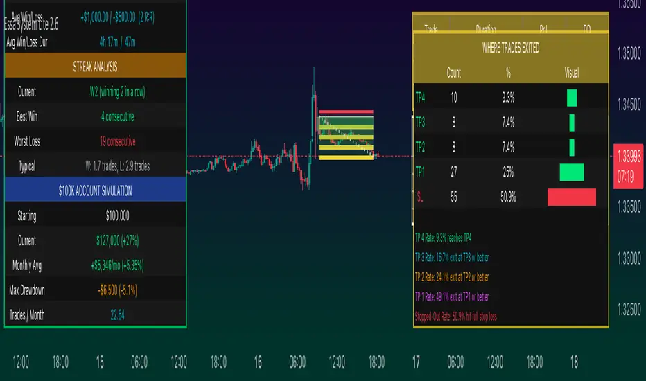
ATR Bands with ATR Cross + InfoTableOverview
This Pine Script™ indicator is designed to enhance traders' ability to analyze market volatility, trend direction, and position sizing directly on their TradingView charts. By plotting Average True Range (ATR) bands anchored at the OHLC4 price, displaying crossover labels, and providing a comprehensive information table, this tool offers a multifaceted approach to technical analysis.
Key Features:
ATR Bands Anchored at OHLC4: Visual representation of short-term and long-term volatility bands centered around the average price.
OHLC4 Dotted Line: A dotted line representing the average of Open, High, Low, and Close prices.
ATR Cross Labels: Visual cues indicating when short-term volatility exceeds long-term volatility and vice versa.
Information Table: Displays real-time data on market volatility, calculated position size based on risk parameters, and trend direction relative to the 20-period Smoothed Moving Average (SMMA).
Purpose
The primary purpose of this indicator is to:
Assess Market Volatility: By comparing short-term and long-term ATR values, traders can gauge the current volatility environment.
Determine Optimal Position Sizing: A calculated position size based on user-defined risk parameters helps in effective risk management.
Identify Trend Direction: Comparing the current price to the 20-period SMMA assists in determining the prevailing market trend.
Enhance Decision-Making: Visual cues and real-time data enable traders to make informed trading decisions with greater confidence.
How It Works
1. ATR Bands Anchored at OHLC4
Average True Range (ATR) Calculations
Short-Term ATR (SA): Calculated over a 9-period using ta.atr(9).
Long-Term ATR (LA): Calculated over a 21-period using ta.atr(21).
Plotting the Bands
OHLC4 Dotted Line: Plotted using small circles to simulate a dotted line due to Pine Script limitations.
ATR(9) Bands: Plotted in blue with semi-transparent shading.
ATR(21) Bands: Plotted in orange with semi-transparent shading.
Overlap: Bands can overlap, providing visual insights into changes in volatility.
2. ATR Cross Labels
Crossover Detection:
SA > LA: Indicates increasing short-term volatility.
Detected using ta.crossover(SA, LA).
A green upward label "SA>LA" is plotted below the bar.
SA < LA: Indicates decreasing short-term volatility.
Detected using ta.crossunder(SA, LA).
A red downward label "SA LA, then the market is considered volatile.
Display: Shows "Yes" or "No" based on the comparison.
b. Position Size Calculation
Risk Total Amount: User-defined input representing the total capital at risk.
Risk per 1 Stock: User-defined input representing the risk associated with one unit of the asset.
Purpose: Helps traders determine the appropriate position size based on their risk tolerance and current market volatility.
c. Is Price > 20 SMMA?
SMMA Calculation:
Calculated using a 20-period Smoothed Moving Average with ta.rma(close, 20).
Logic: If the current close price is above the SMMA, the trend is considered upward.
Display: Shows "Yes" or "No" based on the comparison.
How to Use
Step 1: Add the Indicator to Your Chart
Copy the Script: Copy the entire Pine Script code into the TradingView Pine Editor.
Save and Apply: Save the script and click "Add to Chart."
Step 2: Configure Inputs
Risk Parameters: Adjust the "Risk Total Amount" and "Risk per 1 Stock" in the indicator settings to match your personal risk management strategy.
Step 3: Interpret the Visuals
ATR Bands
Width of Bands: Wider bands indicate higher volatility; narrower bands indicate lower volatility.
Band Overlap: Pay attention to areas where the blue and orange bands diverge or converge.
OHLC4 Dotted Line
Serves as a central reference point for the ATR bands.
Helps visualize the average price around which volatility is measured.
ATR Cross Labels
"SA>LA" Label:
Indicates short-term volatility is increasing relative to long-term volatility.
May signal potential breakout or trend acceleration.
"SA 20 SMMA?
Use this to confirm trend direction before entering or exiting trades.
Practical Example
Imagine you are analyzing a stock and notice the following:
ATR(9) Crosses Above ATR(21):
A green "SA>LA" label appears.
The info table shows "Yes" for "Is ATR-based price volatile."
Position Size:
Based on your risk parameters, the position size is calculated.
Price Above 20 SMMA:
The info table shows "Yes" for "Is price > 20 SMMA."
Interpretation:
The market is experiencing increasing short-term volatility.
The trend is upward, as the price is above the 20 SMMA.
You may consider entering a long position, using the calculated position size to manage risk.
Customization
Colors and Transparency:
Adjust the colors of the bands and labels to suit your preferences.
Risk Parameters:
Modify the default values for risk amounts in the inputs.
Moving Average Period:
Change the SMMA period if desired.
Limitations and Considerations
Lagging Indicators: ATR and SMMA are lagging indicators and may not predict future price movements.
Market Conditions: The effectiveness of this indicator may vary across different assets and market conditions.
Risk of Overfitting: Relying solely on this indicator without considering other factors may lead to suboptimal trading decisions.
Conclusion
This indicator combines essential elements of technical analysis to provide a comprehensive tool for traders. By visualizing ATR bands anchored at the OHLC4, indicating volatility crossovers, and providing real-time data on position sizing and trend direction, it aids in making informed trading decisions.
Whether you're a novice trader looking to understand market volatility or an experienced trader seeking to refine your strategy, this indicator offers valuable insights directly on your TradingView charts.
Code Summary
The script is written in Pine Script™ version 5 and includes:
Calculations for OHLC4, ATRs, Bands, SMMA:
Uses built-in functions like ta.atr() and ta.rma() for calculations.
Plotting Functions:
plotshape() for the OHLC4 dotted line.
plot() and fill() for the ATR bands.
Crossover Detection:
ta.crossover() and ta.crossunder() for detecting ATR crosses.
Labeling Crossovers:
label.new() to place informative labels on the chart.
Information Table Creation:
table.new() to create the table.
table.cell() to populate it with data.
Acknowledgments
ATR and SMMA Concepts: Built upon standard technical analysis concepts widely used in trading.
Pine Script™: Leveraged the capabilities of Pine Script™ version 5 for advanced charting and analysis.
Note: Always test any indicator thoroughly and consider combining it with other forms of analysis before making trading decisions. Trading involves risk, and past performance is not indicative of future results.
Happy Trading!
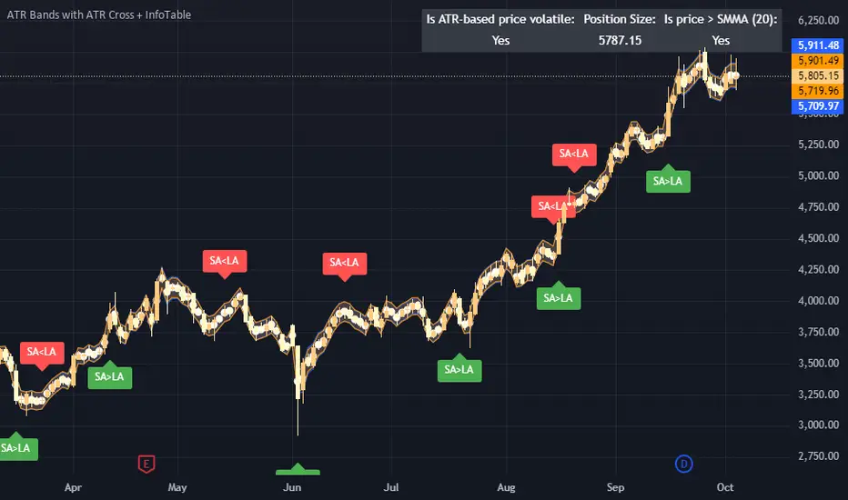
RSI Overbought/Oversold + Divergence Indicator (new)//@version=5
indicator('CryptoSignalScanner - RSI Overbought/Oversold + Divergence Indicator (new)',
//---------------------------------------------------------------------------------------------------------------------------------
//--- Define Colors ---------------------------------------------------------------------------------------------------------------
//---------------------------------------------------------------------------------------------------------------------------------
vWhite = #FFFFFF
vViolet = #C77DF3
vIndigo = #8A2BE2
vBlue = #009CDF
vGreen = #5EBD3E
vYellow = #FFB900
vRed = #E23838
longColor = color.green
shortColor = color.red
textColor = color.white
bullishColor = color.rgb(38,166,154,0) //Used in the display table
bearishColor = color.rgb(239,83,79,0) //Used in the display table
nomatchColor = color.silver //Used in the display table
//---------------------------------------------------------------------------------------------------------------------------------------------------------------------
//--- Functions--------------------------------------------------------------------------------------------------------------------------------------------------------
//---------------------------------------------------------------------------------------------------------------------------------------------------------------------
TF2txt(TF) =>
switch TF
"S" => "RSI 1s:"
"5S" => "RSI 5s:"
"10S" => "RSI 10s:"
"15S" => "RSI 15s:"
"30S" => "RSI 30s"
"1" => "RSI 1m:"
"3" => "RSI 3m:"
"5" => "RSI 5m:"
"15" => "RSI 15m:"
"30" => "RSI 30m"
"45" => "RSI 45m"
"60" => "RSI 1h:"
"120" => "RSI 2h:"
"180" => "RSI 3h:"
"240" => "RSI 4h:"
"480" => "RSI 8h:"
"D" => "RSI 1D:"
"1D" => "RSI 1D:"
"2D" => "RSI 2D:"
"3D" => "RSI 2D:"
"3D" => "RSI 3W:"
"W" => "RSI 1W:"
"1W" => "RSI 1W:"
"M" => "RSI 1M:"
"1M" => "RSI 1M:"
"3M" => "RSI 3M:"
"6M" => "RSI 6M:"
"12M" => "RSI 12M:"
//---------------------------------------------------------------------------------------------------------------------------------------------------------------------
//--- Show/Hide Settings ----------------------------------------------------------------------------------------------------------------------------------------------
//---------------------------------------------------------------------------------------------------------------------------------------------------------------------
rsiShowInput = input(true, title='Show RSI', group='Show/Hide Settings')
maShowInput = input(false, title='Show MA', group='Show/Hide Settings')
showRSIMAInput = input(true, title='Show RSIMA Cloud', group='Show/Hide Settings')
rsiBandShowInput = input(true, title='Show Oversold/Overbought Lines', group='Show/Hide Settings')
rsiBandExtShowInput = input(true, title='Show Oversold/Overbought Extended Lines', group='Show/Hide Settings')
rsiHighlightShowInput = input(true, title='Show Oversold/Overbought Highlight Lines', group='Show/Hide Settings')
DivergenceShowInput = input(true, title='Show RSI Divergence Labels', group='Show/Hide Settings')
//---------------------------------------------------------------------------------------------------------------------------------------------------------------------
//--- Table Settings --------------------------------------------------------------------------------------------------------------------------------------------------
//---------------------------------------------------------------------------------------------------------------------------------------------------------------------
rsiShowTable = input(true, title='Show RSI Table Information box', group="RSI Table Settings")
rsiTablePosition = input.string(title='Location', defval='middle_right', options= , group="RSI Table Settings", inline='1')
rsiTextSize = input.string(title=' Size', defval='small', options= , group="RSI Table Settings", inline='1')
rsiShowTF1 = input(true, title='Show TimeFrame1', group="RSI Table Settings", inline='tf1')
rsiTF1 = input.timeframe("15", title=" Time", group="RSI Table Settings", inline='tf1')
rsiShowTF2 = input(true, title='Show TimeFrame2', group="RSI Table Settings", inline='tf2')
rsiTF2 = input.timeframe("60", title=" Time", group="RSI Table Settings", inline='tf2')
rsiShowTF3 = input(true, title='Show TimeFrame3', group="RSI Table Settings", inline='tf3')
rsiTF3 = input.timeframe("240", title=" Time", group="RSI Table Settings", inline='tf3')
rsiShowTF4 = input(true, title='Show TimeFrame4', group="RSI Table Settings", inline='tf4')
rsiTF4 = input.timeframe("D", title=" Time", group="RSI Table Settings", inline='tf4')
rsiShowHist = input(true, title='Show RSI Historical Columns', group="RSI Table Settings", tooltip='Show the information of the 2 previous closed candles')
//---------------------------------------------------------------------------------------------------------------------------------------------------------------------
//--- RSI Input Settings ----------------------------------------------------------------------------------------------------------------------------------------------
//---------------------------------------------------------------------------------------------------------------------------------------------------------------------
rsiSourceInput = input.source(close, 'Source', group='RSI Settings')
rsiLengthInput = input.int(14, minval=1, title='RSI Length', group='RSI Settings', tooltip='Here we set the RSI lenght')
rsiColorInput = input.color(#26a69a, title="RSI Color", group='RSI Settings')
rsimaColorInput = input.color(#ef534f, title="RSIMA Color", group='RSI Settings')
rsiBandColorInput = input.color(#787B86, title="RSI Band Color", group='RSI Settings')
rsiUpperBandExtInput = input.int(title='RSI Overbought Extended Line', defval=80, minval=50, maxval=100, group='RSI Settings')
rsiUpperBandInput = input.int(title='RSI Overbought Line', defval=70, minval=50, maxval=100, group='RSI Settings')
rsiLowerBandInput = input.int(title='RSI Oversold Line', defval=30, minval=0, maxval=50, group='RSI Settings')
rsiLowerBandExtInput = input.int(title='RSI Oversold Extended Line', defval=20, minval=0, maxval=50, group='RSI Settings')
//---------------------------------------------------------------------------------------------------------------------------------------------------------------------
//--- MA Input Settings -----------------------------------------------------------------------------------------------------------------------------------------------
//---------------------------------------------------------------------------------------------------------------------------------------------------------------------
maTypeInput = input.string("EMA", title="MA Type", options= , group="MA Settings")
maLengthInput = input.int(14, title="MA Length", group="MA Settings")
maColorInput = input.color(color.yellow, title="MA Color", group='MA Settings') //#7E57C2
//---------------------------------------------------------------------------------------------------------------------------------------------------------------------
//--- Divergence Input Settings ---------------------------------------------------------------------------------------------------------------------------------------
//---------------------------------------------------------------------------------------------------------------------------------------------------------------------
lbrInput = input(title="Pivot Lookback Right", defval=2, group='RSI Divergence Settings')
lblInput = input(title="Pivot Lookback Left", defval=2, group='RSI Divergence Settings')
lbRangeMaxInput = input(title="Max of Lookback Range", defval=10, group='RSI Divergence Settings')
lbRangeMinInput = input(title="Min of Lookback Range", defval=2, group='RSI Divergence Settings')
plotBullInput = input(title="Plot Bullish", defval=true, group='RSI Divergence Settings')
plotHiddenBullInput = input(title="Plot Hidden Bullish", defval=true, group='RSI Divergence Settings')
plotBearInput = input(title="Plot Bearish", defval=true, group='RSI Divergence Settings')
plotHiddenBearInput = input(title="Plot Hidden Bearish", defval=true, group='RSI Divergence Settings')
//---------------------------------------------------------------------------------------------------------------------------------------------------------------------
//--- RSI Calculation -------------------------------------------------------------------------------------------------------------------------------------------------
//---------------------------------------------------------------------------------------------------------------------------------------------------------------------
rsi = ta.rsi(rsiSourceInput, rsiLengthInput)
rsiprevious = rsi
= request.security(syminfo.tickerid, rsiTF1, [rsi, rsi , rsi ], lookahead=barmerge.lookahead_on)
= request.security(syminfo.tickerid, rsiTF2, [rsi, rsi , rsi ], lookahead=barmerge.lookahead_on)
= request.security(syminfo.tickerid, rsiTF3, [rsi, rsi , rsi ], lookahead=barmerge.lookahead_on)
= request.security(syminfo.tickerid, rsiTF4, [rsi, rsi , rsi ], lookahead=barmerge.lookahead_on)
//---------------------------------------------------------------------------------------------------------------------------------------------------------------------
//--- MA Calculation -------------------------------------------------------------------------------------------------------------------------------------------------
//---------------------------------------------------------------------------------------------------------------------------------------------------------------------
ma(source, length, type) =>
switch type
"SMA" => ta.sma(source, length)
"Bollinger Bands" => ta.sma(source, length)
"EMA" => ta.ema(source, length)
"SMMA (RMA)" => ta.rma(source, length)
"WMA" => ta.wma(source, length)
"VWMA" => ta.vwma(source, length)
rsiMA = ma(rsi, maLengthInput, maTypeInput)
rsiMAPrevious = rsiMA
//---------------------------------------------------------------------------------------------------------------------------------------------------------------------
//--- Stoch RSI Settings + Calculation --------------------------------------------------------------------------------------------------------------------------------
//---------------------------------------------------------------------------------------------------------------------------------------------------------------------
showStochRSI = input(false, title="Show Stochastic RSI", group='Stochastic RSI Settings')
smoothK = input.int(title="Stochastic K", defval=3, minval=1, maxval=10, group='Stochastic RSI Settings')
smoothD = input.int(title="Stochastic D", defval=4, minval=1, maxval=10, group='Stochastic RSI Settings')
lengthRSI = input.int(title="Stochastic RSI Lenght", defval=14, minval=1, group='Stochastic RSI Settings')
lengthStoch = input.int(title="Stochastic Lenght", defval=14, minval=1, group='Stochastic RSI Settings')
colorK = input.color(color.rgb(41,98,255,0), title="K Color", group='Stochastic RSI Settings', inline="1")
colorD = input.color(color.rgb(205,109,0,0), title="D Color", group='Stochastic RSI Settings', inline="1")
StochRSI = ta.rsi(rsiSourceInput, lengthRSI)
k = ta.sma(ta.stoch(StochRSI, StochRSI, StochRSI, lengthStoch), smoothK) //Blue Line
d = ta.sma(k, smoothD) //Red Line
//---------------------------------------------------------------------------------------------------------------------------------------------------------------------
//--- Divergence Settings ------------------------------------------------------------------------------------------------------------------------------------------
//---------------------------------------------------------------------------------------------------------------------------------------------------------------------
bearColor = color.red
bullColor = color.green
hiddenBullColor = color.new(color.green, 50)
hiddenBearColor = color.new(color.red, 50)
//textColor = color.white
noneColor = color.new(color.white, 100)
osc = rsi
plFound = na(ta.pivotlow(osc, lblInput, lbrInput)) ? false : true
phFound = na(ta.pivothigh(osc, lblInput, lbrInput)) ? false : true
_inRange(cond) =>
bars = ta.barssince(cond == true)
lbRangeMinInput <= bars and bars <= lbRangeMaxInput
//---------------------------------------------------------------------------------------------------------------------------------------------------------------------
//--- Define Plot & Line Colors ---------------------------------------------------------------------------------------------------------------------------------------
//---------------------------------------------------------------------------------------------------------------------------------------------------------------------
rsiColor = rsi >= rsiMA ? rsiColorInput : rsimaColorInput
//---------------------------------------------------------------------------------------------------------------------------------------------------------------------
//--- Plot Lines ------------------------------------------------------------------------------------------------------------------------------------------------------
//---------------------------------------------------------------------------------------------------------------------------------------------------------------------
// Create a horizontal line at a specific price level
myLine = line.new(bar_index , 75, bar_index, 75, color = color.rgb(187, 14, 14), width = 2)
bottom = line.new(bar_index , 50, bar_index, 50, color = color.rgb(223, 226, 28), width = 2)
mymainLine = line.new(bar_index , 60, bar_index, 60, color = color.rgb(13, 154, 10), width = 3)
hline(50, title='RSI Baseline', color=color.new(rsiBandColorInput, 50), linestyle=hline.style_solid, editable=false)
hline(rsiBandExtShowInput ? rsiUpperBandExtInput : na, title='RSI Upper Band', color=color.new(rsiBandColorInput, 10), linestyle=hline.style_dashed, editable=false)
hline(rsiBandShowInput ? rsiUpperBandInput : na, title='RSI Upper Band', color=color.new(rsiBandColorInput, 10), linestyle=hline.style_dashed, editable=false)
hline(rsiBandShowInput ? rsiLowerBandInput : na, title='RSI Upper Band', color=color.new(rsiBandColorInput, 10), linestyle=hline.style_dashed, editable=false)
hline(rsiBandExtShowInput ? rsiLowerBandExtInput : na, title='RSI Upper Band', color=color.new(rsiBandColorInput, 10), linestyle=hline.style_dashed, editable=false)
bgcolor(rsiHighlightShowInput ? rsi >= rsiUpperBandExtInput ? color.new(rsiColorInput, 70) : na : na, title="Show Extended Oversold Highlight", editable=false)
bgcolor(rsiHighlightShowInput ? rsi >= rsiUpperBandInput ? rsi < rsiUpperBandExtInput ? color.new(#64ffda, 90) : na : na: na, title="Show Overbought Highlight", editable=false)
bgcolor(rsiHighlightShowInput ? rsi <= rsiLowerBandInput ? rsi > rsiLowerBandExtInput ? color.new(#F43E32, 90) : na : na : na, title="Show Extended Oversold Highlight", editable=false)
bgcolor(rsiHighlightShowInput ? rsi <= rsiLowerBandInput ? color.new(rsimaColorInput, 70) : na : na, title="Show Oversold Highlight", editable=false)
maPlot = plot(maShowInput ? rsiMA : na, title='MA', color=color.new(maColorInput,0), linewidth=1)
rsiMAPlot = plot(showRSIMAInput ? rsiMA : na, title="RSI EMA", color=color.new(rsimaColorInput,0), editable=false, display=display.none)
rsiPlot = plot(rsiShowInput ? rsi : na, title='RSI', color=color.new(rsiColor,0), linewidth=1)
fill(rsiPlot, rsiMAPlot, color=color.new(rsiColor, 60), title="RSIMA Cloud")
plot(showStochRSI ? k : na, title='Stochastic K', color=colorK, linewidth=1)
plot(showStochRSI ? d : na, title='Stochastic D', color=colorD, linewidth=1)
//---------------------------------------------------------------------------------------------------------------------------------------------------------------------
//--- Plot Divergence -------------------------------------------------------------------------------------------------------------------------------------------------
//---------------------------------------------------------------------------------------------------------------------------------------------------------------------
// Regular Bullish
// Osc: Higher Low
oscHL = osc > ta.valuewhen(plFound, osc , 1) and _inRange(plFound )
// Price: Lower Low
priceLL = low < ta.valuewhen(plFound, low , 1)
bullCond = plotBullInput and priceLL and oscHL and plFound
plot(
plFound ? osc : na,
offset=-lbrInput,
title="Regular Bullish",
linewidth=2,
color=(bullCond ? bullColor : noneColor)
)
plotshape(
DivergenceShowInput ? bullCond ? osc : na : na,
offset=-lbrInput,
title="Regular Bullish Label",
text=" Bull ",
style=shape.labelup,
location=location.absolute,
color=bullColor,
textcolor=textColor
)
//------------------------------------------------------------------------------
// Hidden Bullish
// Osc: Lower Low
oscLL = osc < ta.valuewhen(plFound, osc , 1) and _inRange(plFound )
// Price: Higher Low
priceHL = low > ta.valuewhen(plFound, low , 1)
hiddenBullCond = plotHiddenBullInput and priceHL and oscLL and plFound
plot(
plFound ? osc : na,
offset=-lbrInput,
title="Hidden Bullish",
linewidth=2,
color=(hiddenBullCond ? hiddenBullColor : noneColor)
)
plotshape(
DivergenceShowInput ? hiddenBullCond ? osc : na : na,
offset=-lbrInput,
title="Hidden Bullish Label",
text=" H Bull ",
style=shape.labelup,
location=location.absolute,
color=bullColor,
textcolor=textColor
)
//------------------------------------------------------------------------------
// Regular Bearish
// Osc: Lower High
oscLH = osc < ta.valuewhen(phFound, osc , 1) and _inRange(phFound )
// Price: Higher High
priceHH = high > ta.valuewhen(phFound, high , 1)
bearCond = plotBearInput and priceHH and oscLH and phFound
plot(
phFound ? osc : na,
offset=-lbrInput,
title="Regular Bearish",
linewidth=2,
color=(bearCond ? bearColor : noneColor)
)
plotshape(
DivergenceShowInput ? bearCond ? osc : na : na,
offset=-lbrInput,
title="Regular Bearish Label",
text=" Bear ",
style=shape.labeldown,
location=location.absolute,
color=bearColor,
textcolor=textColor
)
//------------------------------------------------------------------------------
// Hidden Bearish
// Osc: Higher High
oscHH = osc > ta.valuewhen(phFound, osc , 1) and _inRange(phFound )
// Price: Lower High
priceLH = high < ta.valuewhen(phFound, high , 1)
hiddenBearCond = plotHiddenBearInput and priceLH and oscHH and phFound
plot(
phFound ? osc : na,
offset=-lbrInput,
title="Hidden Bearish",
linewidth=2,
color=(hiddenBearCond ? hiddenBearColor : noneColor)
)
plotshape(
DivergenceShowInput ? hiddenBearCond ? osc : na : na,
offset=-lbrInput,
title="Hidden Bearish Label",
text=" H Bear ",
style=shape.labeldown,
location=location.absolute,
color=bearColor,
textcolor=textColor
)
//---------------------------------------------------------------------------------------------------------------------------------------------------------------------
//--- Check RSI Lineup ------------------------------------------------------------------------------------------------------------------------------------------------
//---------------------------------------------------------------------------------------------------------------------------------------------------------------------
bullTF = rsi > rsi and rsi > rsi
bearTF = rsi < rsi and rsi < rsi
bullTF1 = rsi1 > rsi1_1 and rsi1_1 > rsi1_2
bearTF1 = rsi1 < rsi1_1 and rsi1_1 < rsi1_2
bullTF2 = rsi2 > rsi2_1 and rsi2_1 > rsi2_2
bearTF2 = rsi2 < rsi2_1 and rsi2_1 < rsi2_2
bullTF3 = rsi3 > rsi3_1 and rsi3_1 > rsi3_2
bearTF3 = rsi3 < rsi3_1 and rsi3_1 < rsi3_2
bullTF4 = rsi4 > rsi4_1 and rsi4_1 > rsi4_2
bearTF4 = rsi4 < rsi4_1 and rsi4_1 < rsi4_2
bbTxt(bull,bear) =>
bull ? "BULLISH" : bear ? "BEARISCH" : 'NO LINEUP'
bbColor(bull,bear) =>
bull ? bullishColor : bear ? bearishColor : nomatchColor
newTC(tBox, col, row, txt, width, txtColor, bgColor, txtHA, txtSize) =>
table.cell(table_id=tBox,column=col, row=row, text=txt, width=width,text_color=txtColor,bgcolor=bgColor, text_halign=txtHA, text_size=txtSize)
//---------------------------------------------------------------------------------------------------------------------------------------------------------------------
//--- Define RSI Table Setting ----------------------------------------------------------------------------------------------------------------------------------------
//---------------------------------------------------------------------------------------------------------------------------------------------------------------------
width_c0 = 0
width_c1 = 0
if rsiShowTable
var tBox = table.new(position=rsiTablePosition, columns=5, rows=6, bgcolor=color.rgb(18,22,33,50), frame_color=color.black, frame_width=1, border_color=color.black, border_width=1)
newTC(tBox, 0,1,"RSI Current",width_c0,color.orange,color.rgb(0,0,0,100),'right',rsiTextSize)
newTC(tBox, 1,1,str.format(" {0,number,#.##} ", rsi),width_c0,vWhite,rsi < 50 ? bearishColor:bullishColor,'left',rsiTextSize)
newTC(tBox, 4,1,bbTxt(bullTF, bearTF),width_c0,vWhite,bbColor(bullTF, bearTF),'center',rsiTextSize)
if rsiShowHist
newTC(tBox, 2,1,str.format(" {0,number,#.##} ", rsi ),width_c0,vWhite,rsi < 50 ? bearishColor:bullishColor,'left',rsiTextSize)
newTC(tBox, 3,1,str.format(" {0,number,#.##} ", rsi ),width_c0,vWhite,rsi < 50 ? bearishColor:bullishColor,'left',rsiTextSize)
if rsiShowTF1
newTC(tBox, 0,2,TF2txt(rsiTF1),width_c0,vWhite,color.rgb(0,0,0,100),'right',rsiTextSize)
newTC(tBox, 1,2,str.format(" {0,number,#.##} ", rsi1),width_c0,vWhite,rsi1 < 50 ? bearishColor:bullishColor,'left',rsiTextSize)
newTC(tBox, 4,2,bbTxt(bullTF1, bearTF1),width_c0,vWhite,bbColor(bullTF1,bearTF1),'center',rsiTextSize)
if rsiShowHist
newTC(tBox, 2,2,str.format(" {0,number,#.##} ", rsi1_1),width_c0,vWhite,rsi1_1 < 50 ? bearishColor:bullishColor,'left',rsiTextSize)
newTC(tBox, 3,2,str.format(" {0,number,#.##} ", rsi1_2),width_c0,vWhite,rsi1_2 < 50 ? bearishColor:bullishColor,'left',rsiTextSize)
if rsiShowTF2
newTC(tBox, 0,3,TF2txt(rsiTF2),width_c0,vWhite,color.rgb(0,0,0,100),'right',rsiTextSize)
newTC(tBox, 1,3,str.format(" {0,number,#.##} ", rsi2),width_c0,vWhite,rsi2 < 50 ? bearishColor:bullishColor,'left',rsiTextSize)
newTC(tBox, 4,3,bbTxt(bullTF2, bearTF2),width_c0,vWhite,bbColor(bullTF2,bearTF2),'center',rsiTextSize)
if rsiShowHist
newTC(tBox, 2,3,str.format(" {0,number,#.##} ", rsi2_1),width_c0,vWhite,rsi2_1 < 50 ? bearishColor:bullishColor,'left',rsiTextSize)
newTC(tBox, 3,3,str.format(" {0,number,#.##} ", rsi2_2),width_c0,vWhite,rsi2_2 < 50 ? bearishColor:bullishColor,'left',rsiTextSize)
if rsiShowTF3
newTC(tBox, 0,4,TF2txt(rsiTF3),width_c0,vWhite,color.rgb(0,0,0,100),'right',rsiTextSize)
newTC(tBox, 1,4,str.format(" {0,number,#.##} ", rsi3),width_c0,vWhite,rsi3 < 50 ? bearishColor:bullishColor,'left',rsiTextSize)
newTC(tBox, 4,4,bbTxt(bullTF3, bearTF3),width_c0,vWhite,bbColor(bullTF3,bearTF3),'center',rsiTextSize)
if rsiShowHist
newTC(tBox, 2,4,str.format(" {0,number,#.##} ", rsi3_1),width_c0,vWhite,rsi3_1 < 50 ? bearishColor:bullishColor,'left',rsiTextSize)
newTC(tBox, 3,4,str.format(" {0,number,#.##} ", rsi3_2),width_c0,vWhite,rsi3_2 < 50 ? bearishColor:bullishColor,'left',rsiTextSize)
if rsiShowTF4
newTC(tBox, 0,5,TF2txt(rsiTF4),width_c0,vWhite,color.rgb(0,0,0,100),'right',rsiTextSize)
newTC(tBox, 1,5,str.format(" {0,number,#.##} ", rsi4),width_c0,vWhite,rsi4 < 50 ? bearishColor:bullishColor,'left',rsiTextSize)
newTC(tBox, 4,5,bbTxt(bullTF4, bearTF4),width_c0,vWhite,bbColor(bullTF4,bearTF4),'center',rsiTextSize)
if rsiShowHist
newTC(tBox, 2,5,str.format(" {0,number,#.##} ", rsi4_1),width_c0,vWhite,rsi4_1 < 50 ? bearishColor:bullishColor,'left',rsiTextSize)
newTC(tBox, 3,5,str.format(" {0,number,#.##} ", rsi4_2),width_c0,vWhite,rsi4_2 < 50 ? bearishColor:bullishColor,'left',rsiTextSize)
//------------------------------------------------------
//--- Alerts -------------------------------------------
//------------------------------------------------------

Triad Trade MatrixOverview
Triad Trade Matrix is an advanced multi-strategy indicator built using Pine Script v5. It is designed to simultaneously track and display key trading metrics for three distinct trading styles on a single chart:
Swing Trading (Swing Supreme):
This mode captures longer-term trends and is designed for trades that typically span several days. It uses customizable depth and deviation parameters to determine swing signals.
Day Trading (Day Blaze):
This mode focuses on intraday price movements. It generates signals that are intended to be executed within a single trading session. The parameters for depth and deviation are tuned to capture more frequent, shorter-term moves.
Scalping (Scalp Surge):
This mode is designed for very short-term trades where quick entries and exits are key. It uses more sensitive parameters to detect rapid price movements suitable for scalping strategies.
Each trading style is represented by its own merged table that displays real-time metrics. The tables update automatically as new trading signals are generated.
Key Features
Multi-Style Tracking:
Swing Supreme (Large): For swing trading; uses a purple theme.
Day Blaze (Medium): For day trading; uses an orange theme.
Scalp Surge (Small): For scalping; uses a green theme.
Real-Time Metrics:
Each table displays key trade metrics including:
Entry Price: The price at which the trade was entered.
Exit Price: The price at which the previous trade was exited.
Position Size: Calculated as the account size divided by the entry price.
Direction: Indicates whether the trade is “Up” (long) or “Down” (short).
Time: The time when the trade was executed (formatted to hours and minutes).
Wins/Losses: The cumulative number of winning and losing trades.
Current Price & PnL: The current price on the chart and the profit/loss computed relative to the entry price.
Duration: The number of bars that the trade has been open.
History Column: A merged summary column that shows the most recent trade’s details (entry, exit, and result).
Customizability:
Column Visibility: Users can toggle individual columns (Ticker, Timeframe, Entry, Exit, etc.) on or off according to their preference.
Appearance Settings: You can customize the table border width, frame color, header background, and text colors.
History Toggle: The merged history column can be enabled or disabled.
Chart Markers: There is an option to show or hide chart markers (labels and lines) that indicate trade entries and exits on the chart.
Trade History Management:
The indicator maintains a rolling history (up to three recent trades per trading style) and displays the latest summary in the merged table.
This history column provides a quick reference to recent performance.
How It Works
Signal Generation & Trade Metrics
Trade Entry/Exit Calculation:
For each trading style, the indicator uses built-in functions (such as ta.lowestbars and ta.highestbars) to analyze price movements. Based on a customizable "depth" and "deviation" parameter, it determines the point of entry for a trade.
Swing Supreme: Uses larger depth/deviation values to capture swing trends.
Day Blaze: Uses intermediate values for intraday moves.
Scalp Surge: Uses tighter parameters to pick up rapid price changes.
Metrics Update:
When a new trade signal is generated (i.e., when the trade entry price is updated), the indicator calculates:
The current PnL as the difference between the current price and the entry price (or vice versa, depending on the trade direction).
The duration as the number of bars since the trade was opened.
The position size using the formula: accountSize / entryPrice.
History Recording:
Each time a new trade is triggered (i.e., when the entry price is updated), a summary string is created (showing entry, exit, and win/loss status) and appended to the corresponding trade history array. The merged table then displays the latest summary from this history.
Table Display
Merged Table Structure:
Each trading style (Swing Supreme, Day Blaze, and Scalp Surge) is represented by a table that has 15 columns. The columns are:
Trade Type (e.g., Swing Supreme)
Ticker
Timeframe
Entry Price
Exit Price
Position Size
Direction
Time of Entry
Account Size
Wins
Losses
Current Price
Current PnL
Duration (in bars)
History (the latest trade summary)
User Customization:
Through the settings panel, users can choose which columns to display.
If a column is toggled off, its cells will remain blank, allowing traders to focus on the metrics that matter most to them.
Appearance & Themes:
The table headers and cell backgrounds are customizable via color inputs. The trading style names are color-coded:
Swing Supreme (Large): Uses a purple theme.
Day Blaze (Medium): Uses an orange theme.
Scalp Surge (Small): Uses a green theme.
How to Use the Indicator
Add the Indicator to Your Chart:
Once published, add "Triad Trade Matrix" to your TradingView chart.
Configure the Settings:
Adjust the Account Size to match your trading capital.
Use the Depth and Deviation inputs for each trading style to fine-tune the signal sensitivity.
Toggle the Chart Markers on if you want visual entry/exit markers on the chart.
Customize which columns are visible via the column visibility toggles.
Enable or disable the History Column to show the merged trade history in the table.
Adjust the appearance settings (colors, border width, etc.) to suit your chart background and preferences.
Interpret the Tables:
Swing Supreme:
This table shows metrics for swing trades.
Look for changes in entry price, PnL, and trade duration to monitor longer-term moves.
Day Blaze:
This table tracks day trading activity.It will update more frequently, reflecting intraday trends.
Scalp Surge:
This table is dedicated to scalping signals.Use it to see quick entry/exit data and rapid profit/loss changes.
The History column (if enabled) gives you a snapshot of the most recent trade (e.g., "E:123.45 X:124.00 Up Win").
Use allerts:
The indicator includes alert condition for new trade entries(both long and short)for each trading style.
Summary:
Triad Trade Matrix provides an robust,multi-dimensional view of your trading performance across swing trading, day trading, and scalping.
Best to be used whith my other indicators
True low high
Vma Ext_Adv_CustomTbl
This indicator is ideal for traders who wish to monitor multiple trading styles simultaneously, with a clear, technical, and real-time display of performance metrics.
Happy Trading!

Argentum Flag [AGP] Ver.2.5Central Purpose and Concept
The Argentum Flag script is a multifunctional tool that integrates and visualizes multiple key indicators to provide a detailed and unified perspective of the market. The core concept is to analyze price from different angles—volatility, volume, and momentum—to identify confluences and patterns that may be difficult to see with separate indicators. This "mashup" is not a simple fusion of indicators, but a strategic combination of tools that complement each other to offer a comprehensive view of asset behavior.
Components and Their Functionality
This script combines and visualizes the following elements:
EMA Percentage Bands (EMA Bands):
Uses an Exponential Moving Average (EMA) as a baseline.
Calculates and draws several volatility bands that deviate from the central EMA by fixed percentages (0.47%, 0.94%, 2.36%). These bands are inspired by Fibonacci ratios and the cyclical nature of the market.
The bands are colored with a dynamic gradient that reflects the current state of volatility.
Utility: These bands act as dynamic support and resistance areas. The price entering or exiting these zones can indicate a change in volatility or a possible exhaustion of the movement.
Volatility Signals (Vortex & Prime Signals):
The script generates visual signals when the price stays outside the volatility bands for a specific number of bars.
Vortex Signals (diamond ⍲): Appear when the price crosses and stays outside the Prime bands, suggesting a high volatility or a possible continuation of the trend.
Exit/Entry Signals (circle ⌾): Are activated when the price stays outside the Vortex bands, indicating an extreme extension of volatility. These can be interpreted as potential reversal or profit-taking zones.
Utility: They help traders quickly identify moments of high and low volatility and potential turning points in price action.
Volume Analysis (Volume Bar Colors):
The script changes the color of the bars based on the relationship between the current volume and the average volume over a 50-bar period.
Utility: This feature allows the trader to immediately visualize the strength behind a price movement. For example, a bullish candle with "extreme" volume suggests strong buying interest, while a bearish candle with "low" volume could indicate a weak correction.
Summary Tables (Dashboard):
EMA-Fibo Table: Displays the values of 12 EMAs based on the Fibonacci sequence (5, 8, 13, 21...) in an easy-to-access table. The background color of each value indicates if the current price is above (bullish) or below (bearish) that EMA.
Multi-Timeframe RSI Table: Displays the Relative Strength Index (RSI) values across multiple timeframes (from 1 minute to monthly). The text color changes to highlight if the RSI is in overbought (orange) or oversold (white) areas, according to the established levels.
Utility: These tables condense a large amount of data into a simple format, allowing traders to perform a quick, multi-timeframe market analysis without constantly switching charts.
How to Use the Script
This script is a contextual analysis tool that works best when its different components are combined. It is not a "buy and sell signal" system on its own, but a tool for informed decision-making.
Trend Identification: Use the EMA table to see the general trend direction across different timeframes. A price above most of the EMAs in the table suggests a bullish bias.
Volatility Reading: Observe the EMA bands. If the price stays within the bands, volatility is low. A strong move that breaks out of the bands, accompanied by an "extreme" volume color (blue), suggests strong momentum that could continue.
Momentum Analysis: Use the RSI table to confirm movements. An overbought 15m RSI could support a reversal signal from the Vortex bands, while a 1D RSI in a neutral zone may indicate that the main trend has not changed.
Signal Confirmation: Visual signals (diamond and circle) should not be used in isolation. They must be confirmed by volume analysis and dashboard readings. For example, an "Exit Signal" (circle) with low volume may be less reliable than one with high volume and a clear reversal candle.
Disclaimer
This script is for informational and educational purposes only. It is not financial advice, nor is it a recommendation to buy or sell any financial instrument. All trading involves risk, and past performance is not indicative of future results. The user is solely responsible for their own trading decisions.

Relative Strength and MomentumRelative Strength and Momentum Indicator
Unlock deeper market insights with the Relative Strength and Momentum Indicator—a powerful tool designed to help traders and investors identify the strongest stocks and sectors based on relative performance. This custom indicator displays essential information on relative strength and momentum for up to 15 different symbols, compared against a benchmark index, all within a clear and organized table format.
Key Features:
1. Customizable Inputs: Choose up to 15 symbols to compare, along with a benchmark index, allowing you to tailor the indicator to your trading strategy. The 'Lookback Period' input defines how many weeks of data are analyzed for relative strength and momentum.
2. Relative Strength Calculation: For each selected symbol, the indicator calculates the Relative Strength (RS) against the chosen benchmark. This RS is further refined using an exponential moving average (EMA) to smooth the results, providing a more stable trend overview.
3. Momentum Analysis: Momentum is determined by analyzing the rate of change in relative strength. The indicator calculates a momentum rank for each symbol, based on its relative strength’s improvement or deterioration.
4. Percentile Ranking System: Each symbol is assigned a percentile rank (from 1 to 100) based on its relative strength compared to the others. Similarly, momentum rankings are also assigned from 1 to 100, offering a clear understanding of which assets are outperforming or underperforming.
5. Visual Indicators:
a. Green: Signals improving or stable relative strength and momentum.
b. Red: Indicates declining relative strength or momentum.
c. Aqua: Highlights symbols performing well on both relative strength and momentum—ideal candidates for further analysis.
6. Two Clear Tables:
a. Relative Strength Rank Table: Displays weekly rankings of relative strength for each symbol.
b. Momentum Table: Shows momentum trends, helping you identify which symbols are gaining or losing strength.
7. Color-Coded for Easy Analysis: The tables are color-coded to make analysis quick and straightforward. A green color means the symbol is performing well in terms of relative strength or momentum, while red indicates weaker performance. Aqua marks symbols that are excelling in both areas.
Use Case:
a. Sector Comparison: Identify which sectors or indexes are showing both relative strength and momentum to pick high-potential stocks. This allows you to align with broader market trends for improved trade entries.
b. Stock Selection: Quickly compare symbols within the same sector to find the stronger performers.